
Feeds
KDE Plasma 6.1.5, Bugfix Release for September
Tuesday, 10 September 2024. Today KDE releases a bugfix update to KDE Plasma 6, versioned 6.1.5.
Plasma 6.1 was released in June 2024 with many feature refinements and new modules to complete the desktop experience.
This release adds a month's worth of new translations and fixes from KDE's contributors. The bugfixes are typically small but important and include:
- Screenedge: allow activating clients in drag and drop. Commit. Fixes bug #450579
- Applets/kickoff: Fix keyboard navigation getting stuck inside gridviews. Commit. Fixes bug #489867
- Klipper: fix copying cells when images are ignored. Commit. Fixes bug #491488
Ben Hutchings: FOSS activity in July 2024
- I continued participating in Debian kernel team meetings.
- For the Debian linux package:
- I investigated a regression for nftables introduced in my final upload of linux to buster-security, and passed on the information to the Freexian ELTS team.
- I uploaded:
- linux version 6.1.94-1~bpo11+1 to bullseye-backports.
- linux version 6.8.12-1~bpo12+1 to bookworm-backports.
- linux version 6.9.7-1~bpo12+1 to bookworm-backports.
- linux version 6.10-1~exp1 to experimental.
- linux version 6.1.99-1~bpo11+1 to bullseye-backports (but it was never accepted).
- linux version 6.10.1-1~exp1 to experimental.
- linux version 6.9.10-1~bpo12+1 to bookworm-backports.
- I opened or updated MRs:
- !1077: d/b/gencontrol.py, d/rules.real: Restore config checks on kernels to be signed
- !1112: Update d/l/p/debian_linux/firmware.py for current WHENCE format
- !1115: Update to 6.10-rc7
- !1119: Update d/b/test-patches to work with current package
- !1126: [alpha] scsi: Disable SCSI_IMM (fixes FTBFS)
- !1133: Draft: Fix sh4/sh7785lcr flavour
- I reviewed MRs:
- !675: [arm64] drivers/usb/host: Enable USB_XHCI_PCI_RENESAS as module (Closes: #1032671)
- !732: [x86] linux-cpupower: Add intel-speed-select command
- !957: debian/bin/gencontrol.py: allow adding a custom suffix to the abiname (closed)
- !964: tools/arch/x86/intel_sdsi: Add sdsi package for Intel SDSi provisioning tool
- !1037: debian/rules.real: set absolute bpftool path for linux 6.8+ (closed)
- !1038: debian/rules.real: export LANG = C.UTF-8 for sphinx
- !1041: Add “-b” flag to genorig.py
- !1051: [x86] drivers/platform/x86: Enable MSI_EC as module (merged)
- !1059: [amd64/cloud] drivers/watchdog: Enable I6300ESB_WDT as module (merged)
- !1074: MIPS64EL: add mips64r6el flavor (merged)
- !1084: Remove unused check for image size
- !1093: d/rules.d/t/perf/Makefile: Enable debuginfod support. (merged)
- !1094: [arm64] drivers/gpu/drm/bridge/synopsys: Enable DRM_DW_HDMI_I2S_AUDIO as module (merged)
- !1095: [arm64] Enable config options for Qualcomm boards (merged)
- !1100: kernel/power: enable CONFIG_HIBERNATION_COMP_LZ4
- !1118: [x86] sound/soc/intel/avs/boards: Enable SND_SOC_INTEL_AVS_MACH_MAX98927 as a module (merged)
- !1122: Enable snd_soc_pcm5102a as a module (merged)
- !1123: [ppc64*] Switch default kernel to 4k page size (merged)
- !1128: drivers/md/dm-vdo: Enable DM_VDO as module (merged)
- !1129: Backport Microsoft Azure Network Adapter from 6.10
- !1134: debian/rules: sort control.md5sums to improve reproducibility (merged)
- !1135: [arm64] Re-enable RELR (merged)
- !1136: Compile with gcc-14 on all architectures
- !1139: [arm64] enable CONFIG_QCOM_LMH, another SDM845-related option (merged)
- !1141: drivers/net: Enable NETKIT (BPF-programmable network device)
- !1142: fs/erofs: Enable more EROFS compression algorithms (merged)
- I merged my own MRs:
- !1110: d/l/p/debian_linux/firmware.py: Handle RawFile fields
- !1112: Update d/l/p/debian_linux/firmware.py for current WHENCE format
- !1119: Update d/b/test-patches to work with current package
- !1126: [alpha] scsi: Disable SCSI_IMM (fixes FTBFS)
- To support Debian ELTS, I created branches of the Linux 5.10 and 6.1 packaging with backports of the change to use an ephemeral module signing key.
- I answered a query about use of the linux-image-*-unsigned packages.
- I responded to bug reports:
- #989229: grub-install: warning: Cannot read EFI Boot* variables
- #1039883: linux: ext4 corruption with symlinks
- #1063754: fat-modules: SD corruption upon opening file on Linux desktop
- #1075855: Kernel panic caused by aacraid module prevents normal boot
- #1072063: one of the external monitors randomly blank for 2-3 seconds with 6.8/6.9 Linux kernels (regression)
- #1072311: linux-perf can (and should) link against libdebuginfod
- Upstream, I commented on how to detect 32-bit architectures in order to fix CVE-2024-42258.
- Upstream, I submitted the patch xhci-pci: Make xhci-pci-renesas a proper modular driver which is a prerequisite for merging MR !675.
- I asked the Debian Super-H porters whether the sh7785lcr kernel flavour was useful.
- In dput-ng, I merged my own MR !36: rsync, scp: Fix username lookup.
- In devscripts, I updated and merged my own MR !292: uscan: Allow compression of VCS exports to be disabled. This can make uscan a lot faster for packages that use a VCS as upstream and exclude some files from it.
- For the Debian firmware-nonfree package:
- I opened MRs:
- I reviewed MRs:
- I merged my own MRs:
- !96: Update to 20240610
- !98: Include or exclude most unpackaged firmware
- !101: Update to 20240709 and remove some file exclusions
- I uploaded versions 20240610-1 and 20240709-1 to unstable.
- I responded to bug reports:
- In the kernel-team repository:
- I reviewed MRs:
- I deleted the obsolete script that !2 would have updated.
- For the Debian wireless-regdb package:
- I reviewed MRs:
- !4: merge stretch-elts 2022.04.08-1~deb9u1 upload (closed)
- !5: Upload For LTS (buster) (merged)
- I reviewed MRs:
- For the Debian nfs-utils package:
- I opened MR !31: Fixes for handling of state files in /var/lib/nfs in response to bug #1074359: nfs-kernel-server: Updating package unexports all filesystems, and later merged it.
- I reviewed and merged MR !15: A couple more DEP8 tests.
- For the Debian klibc package:
- For the Debian ktls-utils package:
- I updated to upstream version 0.11 and uploaded version 0.11-1 to unstable.
- For the Debian initramfs-tools package:
- I uploaded version 0.143.1 to unstable, with no changes from version 0.143. One of the changes in 0.143 happened to fix the newly reported #1076539: plymouth: Updating plymouth fails with “No space left on device” (and its many duplicates).
- I reviewed MRs:
- !70: Support MODULES=dep usage when root was mounted from root specified on kernel command line (closed)
- !78: feature: safely close devices on shutdown (closed)
- !84: Allow providing UDEV_WAIT and ROUNDTTT times in environment variables
- !89: init: Remove tmpfs from rootfstype option
- !96: mkinitramfs: Do not store intermediate main cpio archive (merged)
- !107: Replace copy_modules_dir by manual_add_modules calls (merged)
- !116: autopkgtest: Enable KVM if available (merged)
- !117: install hid-multitouch module for Surface Pro 4 Keyboard (merged)
- !118: fsck: Mention file system name in failed identification warning (merged)
- !119: Fix resume device type check
- !120: hook-functions: auto_add_modules: Add onboard_usb_hub, onboard_usb_dev (merged)
- !121: hook-functions: add_loaded_modules: Walk bound devices for suppliers (merged)
- !122: d/gbp.conf: Set gbp-dch options matching existing changelog entries (merged)
- !123: mkinitramfs: Add -m argument to override MODULES setting (merged)
- !124: mkinitramfs: Add MODULES=all option to add every module (closed)
- !126: Move shellcheck configuration to .shellcheckrc (merged)
- I responded to bug reports:
- #961395: initramfs-tools: failed hardlink initrd.img
- #980021: initramfs-tools: Upgrading a LVM2 system with separate /usr to buster breaks booting
- #1027749: update-initramfs could diagnose attempt to run with /dev not mounted
- #1054991: initramfs-tools: failed to make backup on esp directory /boot
- #1065698: update-initramfs: -k all stopped working
- #1068195: USB keyboard unusable when booting with init=/bin/bash
- I reported Debian bugs:
- For the Debian a56 package, which is a build-dependency of firmware-free, I made an NMU fixing a build failure with gcc-14 and many compiler warnings. These changes were included in version 1.3+dfsg-11.
ImageX: Test and Publish Easily: Exclusive Drupal Content Management Options with the Workspaces Module
Authored by Nadiia Nykolaichuk.
Having your website on the World Wide Web is a responsible task because it must always be impeccable in the eyes of your audience. What if you must launch a new product, run a content-rich campaign, or just review and publish large amounts of content?
Talking Drupal: Talking Drupal #466 - Progressive Migration
Today we are talking about Progressive migration with Drupal, What it is, and how you can do it with your organization with guest Stephen Cross. We’ll also cover Views JSON Source as our module of the week.
For show notes visit: www.talkingDrupal.com/466
Topics- What is a progressive migration
- What other types of migration are there
- What problem does progressive migration solve at the ATF
- What versions of Drupal are involved
- Technical implementation
- Technical challenges
- Non-Technical challenges
- Processes needed for success
- When to use another migration process
- Drupal GovCon Presentation - Progressive Migration
- Talking Drupal #334 - Managing Drupal Teams in Government
Stephen Cross - stephencross.com stephencross
HostsNic Laflin - nLighteneddevelopment.com nicxvan John Picozzi - epam.com johnpicozzi Nate Dentzau - dentzau.com nathandentzau
MOTW CorrespondentMartin Anderson-Clutz - mandclu.com mandclu
- Brief description:
- Have you ever wanted to use Drupal’s Views interface to allow visitors to browse and navigate data from another source? There’s a module for that
- Module name/project name:
- Brief history
- How old: created in Apr 2020 by Pradeep Venugopal (venugopp), but recent releases are by Viktor Holovachek (astonvictor), a member of the Ukraine Drupal community
- Versions available: 2.0.2 compatible with Drupal 8.8 and newer, all the way up to Drupal 11
- Maintainership
- Actively maintained
- Security coverage
- Documentation: pretty lengthy README to help you get started
- Number of open issues: 17 open issues, 4 of which are bugs against the current branch, although one had a fixed merged in the past week
- Usage stats:
- 1,641 sites
- Module features and usage
- After installing the module, you can create a view and specify it should show “JSON” instead of some kind of content entity
- In the view settings you can then provide a URL for where to retrieve the JSON, and an optional Apath value to indicate a section of the data to show
- It also supports contextual filters, so you can create a single view that will show different sections of data depending on the path used to access it
- From there you can build out your view in the normal way: using fields to specify what data should be shown and how, filters to limit which rows will be shown, and sort criteria to specify the order in which it will be listed. And of course, the ability to expose controls for users to filter and sort the data in ways that meet their own needs make this an extremely powerful way to make data available to your site’s visitors
- We spoke a couple of episodes ago about how powerful it can be to use Drupal as the “glass” or experience layer through which visitors can interact with other systems, and I think this is another great example of that
Drupal Association blog: Join Us at the Drupal Association Booth at DrupalCon Barcelona!
Drupal is thriving due to the contributions of its community of developers, site builders, designers, business owners, and more. Our open source model ensures that everyone has a voice and can directly contribute to the platform’s growth, making it more powerful, flexible, and secure. In a couple of weeks, our chance to come together in person is not just about learning the latest in Drupal development; it’s about connecting with like-minded individuals who share a passion for open source and the open web.
Some of the crowd attending DrupalCon Portland in May 2024
We welcome all attendees to stop by the Drupal Association booth at DrupalCon Barcelona to share their ideas, meet our team, learn more about our work, and how to get involved. If you’re not already a supporter, you can sign up and discover how your contribution as a Ripple Maker or a Drupal Certified Partner can make a significant impact. Other opportunities are the Drupal Certified Partner Roundtable or the Ripple Makers Roundtable. The Drupal Association is hosting a coffee for Ripple Makers on Wednesday, 25 September at 8:45 am. The first 50 people who RSVP reserve their spot - you can RSVP here!
Other Drupal Association sessions include Bridging the Gap: Unlocking Non-Code Contributions on Wednesday, the Drupal.org Engineering Panel, the Local Drupal Regions & Associations Round Table, and Supply Chain Security in Drupal and Composer on Thursday. Lastly, we also encourage you to attend the Drupal Association Public Board Meeting, also on Thursday. At this session, the community-elected 2024 At-Large Board member will be announced and welcomed onto the board.
Make sure to also ask about Drupal CMS (aka Drupal Starshot) to learn more about the initiative when you’re visiting the Drupal Association booth. We’ll share:
- The latest Drupal CMS news
- Plans for the future of Drupal CMS, especially the first market-ready version
- How you can get involved in helping with this awesome product!
There will also be a giveaway to win one of three Drupal Starshot initiative posters. Visit us at the booth to enter for a chance to win!
DrupalCon is a vibrant, collaborative space where individuals from all walks of life come together to create, innovate, and share. The event fosters friendships, offers inspiration, and provides opportunities to contribute back to the community in meaningful ways. The excitement around Drupal CMS and the energy of being surrounded by people who love Drupal is palpable, making DrupalCon an invaluable experience for both newcomers and seasoned contributors alike.
If you can’t make the event in person, we invite you to become a Ripple Maker or a Drupal Certified Partner. You’re not just making a contribution—you’re investing in the future of Drupal. With increased and customized communication, you will learn how these programs support critical initiatives such as security updates, community events, and educational resources that benefit users and developers alike. With your support, you'll be part of the dedicated group of community members who understand the importance of giving back and ensuring that Drupal remains a powerful, free, and open-source tool for everyone.
See you in Barcelona from 24-27 September 2024!
BRAINSUM: Harnessing the Power of Decoupled Architecture with Next.js and Drupal
In today's digital ecosystem, the choice of technology stack is crucial to the success of any project, particularly when developing large-scale web applications. A trend gaining momentum is the decoupling of the frontend and backend, which enhances flexibility, scalability, and the overall user experience. This architectural choice is brilliantly exemplified by the integration of Next.js and Drupal, where Drupal's robust content management capabilities are combined with the modern frontend framework of Next.js.
Recognizing the limitations of its traditional Twig-based frontend, Drupal has embraced a more flexible approach known as "Decoupled Drupal." This blog post delves into projects that we’ve worked on: Novozymes and Novonesis that leveraged Next.js for the frontend and Drupal as the headless CMS backend, offering valuable insights for digital solution leads and developers keen on exploring this technology stack.
Open Source AI Definition – Weekly update September 9
Week 36 summary
Draft v.0.0.9 of the Open Source AI Definition is available for comments- -@Shamar agrees with @thesteve0 and emphasizes that AI systems consist of two parts: a virtual machine (architecture) and the weights (the executable software). He argues that while weights are important, they are not sufficient to study or fully understand an AI model. For a system to be truly Open Source, it must provide all the data used to recreate an exact copy of the model, including random values used during the process. Without this, the system should not be labeled Open Source, even if the weights are available under an open-source license. Shamar suggests calling such systems “freeware” instead and ensuring the Open Source AI Definition aligns with the Open Source Definition.
- @jberkus questions whether creating an exact copy of an AI system is truly possible, even with access to all the training data, or if slight differences would always exist.
- @shujisado explains that under Japan’s copyright law, AI training on publicly available copyrighted works is permissible, but sharing the datasets created during training requires explicit permission from copyright holders. He notes that while AI training within legal limits may be allowed in many jurisdictions, making all training data freely available is unlikely. He adds that the current Open Source AI Definition strikes a reasonable balance given global intellectual property rights but suggests that more specific language might help clarify this further.
- @marianataglio suggests including hardware specifications, training time, and carbon footprint in the Open Source AI Definition to improve transparency. She believes this would enhance reproducibility, accessibility, and collaboration, while helping practitioners estimate computational costs and optimize models for more efficient training.
- The fifthteenth edition of our town hall meetings was held on the 6th of September. If you missed it, the recording and slides can be found here.
- @Alek_Tarkowski agrees with @arandal on the importance of situating Open Source AI within broader open movements like open data. He suggests cooperation with organizations like Creative Commons should go beyond licensing standards to include data governance, which remains an undeveloped area.
- @Alek_Tarkowski finds the idea of requiring source data to follow Open Source licenses conceptually interesting, likening it to “upstream copyleft,” but notes traditional copyleft frameworks may not suit AI development.
- @arandal clarifies that the proposal is an evolution of software freedom principles, not a direct extension of traditional copyleft, similar to how AGPL addressed gaps left by earlier licenses. They further mention that discussions on these approaches are ongoing across various organizations, though formal publications are limited.
- @Senficon highlights a concern from the open science community that, while EU copyright law allows reproductions of protected content for research, it restricts making the research corpus available to third parties. This limits research reproducibility and open access, as it aims to protect rights holders’ revenue.
- @kjetilk agrees with the observation but questions the assumption that making content publicly available would significantly harm rights holders’ revenue. He believes such policies should be based on solid evidence from extensive research.
The Drop Times: Get Ready for DrupalCon Barcelona 2024: What to Expect
DrupalCon Barcelona is just around the corner, running from September 9 to 12, 2024. As one of the most anticipated events in the Drupal community, this year’s conference promises to deliver a blend of technical insights, community collaboration, and exciting updates that everyone will be talking about. If you're a developer, site builder, project manager, or just someone intrigued by the future of web technology, there’s something in store for you.
Why DrupalCon Barcelona MattersThis year's DrupalCon is packed with key sessions, hands-on workshops, and networking opportunities designed to bring the community together. Whether you’re looking to dive deep into Drupal 11, which will see some significant updates during the event, or catch the latest on how Drupal is evolving as a powerful digital platform, the conference is shaping up to be a can't-miss opportunity.
What’s New? A Focus on StarshotA highlight of the event will be the ongoing work on the Starshot Initiative, which is aimed at taking Drupal to the next level. In a recent interview with The Drop Times, Drupal’s founder Dries Buytaert shared,
"Our next big milestone is DrupalCon Barcelona, which is in September. We hope to show some real progress there on a variety of different things, from marketing to our demo of Starshot to maybe having the first recipes... implemented."
This makes DrupalCon Barcelona not just another tech event but a milestone where the community will witness key advancements, including live demos of Starshot. The first recipes, a crucial technical feature within Starshot, might be unveiled, offering an early glimpse into the future of Drupal.
Program HighlightsThe event's schedule will feature sessions on critical topics such as Composer, security, local development, and the latest updates in Drupal 11. Expect to hear about performance improvements, new modules, and security enhancements that aim to make Drupal 11 even more powerful. Developers will also have the opportunity to discuss workflows, integrations, and DevOps practices that can streamline their projects.
Additionally, keep an eye on the Starshot Initiative sessions, where you’ll get a closer look at how this ambitious project is progressing and what it means for Drupal’s future. We have listed the key Starshot sessions happening at DrupalCon Barcelona—take a look at the Key Sessions on Drupal Starshot Initiative at DrupalCon Barcelona 2024
Community and Networking OpportunitiesAs always, DrupalCon is more than just technical talks. It's about community. The event is set to feature numerous networking events, helping attendees meet fellow Drupal enthusiasts, share ideas, and collaborate on projects. Whether you're looking to expand your skill set or connect with others in the industry, DrupalCon Barcelona offers the perfect platform.
Why You Should AttendWith all the excitement surrounding Starshot and the recent release of Drupal 11, there’s no better place to catch up on the latest developments in the Drupal ecosystem. With keynotes from leading voices in the community, hands-on workshops, and the promise of some surprise updates, DrupalCon Barcelona 2024 is poised to leave a lasting mark.
Don’t miss your chance to be part of this landmark event. Now, as we proceed further, let’s find out what The Drop Times has covered last week:
In an exclusive interview, Vincenzo Gambino, Drupal Architect and Senior React Developer, shared his career journey from Palermo to London with our former sub-editor, Elma John. He discussed working on high-profile projects, such as those for Cambridge University, and co-authoring Jumpstart Jamstack Development. Vincenzo touched on the role of Drupal in headless architectures and its future in open-source technologies.
Christian Burk, Senior Backend Engineer at CivicActions, provided insights into managing complex content changes on large sites like VA.gov during Drupal GovCon 2023. He highlighted the codit_batch_operations module, which simplifies revisions, logging, and script execution alongside co-presenter Steve Wirt.
At the same event, Michael Kinnunen, Backend Engineer at CivicActions, discussed A/B testing within Drupal using LaunchDarkly, underscoring the platform’s versatility for government websites. He also attended sessions on content translation and large-scale content management, deepening his understanding of Drupal's growing influence.
In other news, Drupal CMS has launched a community survey to improve its default search configuration. The initiative, led by 1XINTERNET, focuses on making Drupal’s search functionality more flexible for both developers and no-code users. Community members are encouraged to contribute to shaping the future of Drupal’s search experience.
Additionally, Drupal.org has updated its fonts to enhance readability, switching to ZT Gatha for headings and Noto Sans for body text. The update modernizes the platform’s look, improving user experience across its global community.
For a deep dive into Dresktop, an open-source tool transforming Drupal management, check out a tutorial by José Daniel Estrada Guzmán. From local development to cloud integration, Dresktop streamlines workflows using Docker, SSH, and Drush.
Lukas Fischer, CEO of Netnode AG, shared his innovative Native Design Flow, which integrates Figma and code at the outset of a project. This approach aims to eliminate the traditional design handoff, creating a more cohesive and efficient workflow from day one.
For the first time, local Drupal associations will jointly host a booth, highlighting collaboration within the European Drupal community. The booth will serve as a hub for networking and sharing information about upcoming events.
Looking ahead to other events, the NEDCamp 2024 session submission deadline has been extended to September 15, offering opportunities for presenters of all experience levels. Splash Awards Switzerland 2025 is scheduled for March 11 in Davos, coinciding with Drupal Mountain Camp. These awards celebrate the best in Drupal projects and innovation.
Early bird registration for DrupalCamp Berlin 2024 remains open until September 15, offering a discounted rate of €80. After October 15, the price will increase to €120, so early registration is recommended. The ticket includes entry, lunch, and an official event T-shirt.
Additionally, DrupalSouth Community Day 2024 in Canberra is seeking volunteers for event support, speaker coordination, and attendee assistance. The call for papers is also open, inviting Drupal professionals to submit session proposals for the event on November 14.
Meanwhile, The Splash Awards will debut in Asia at DrupalCon Singapore on December 9, 2024, celebrating excellence in Drupal projects across categories like Government, Corporate, and Education.
Mark your calendars for DrupalCamp Atlanta on October 18, 2024, in Sandy Springs, Georgia. This one-day conference will offer sessions on the technical and business aspects of Drupal and plenty of networking opportunities.
Finally, join The Drop Times at DrupalCon Barcelona as a volunteer to help cover the event’s best moments. From live updates to behind-the-scenes stories, it’s a great way to engage with the community and share the excitement.
We acknowledge that there are more stories to share. However, due to selection constraints, we must pause further exploration for now.
To get timely updates, follow us on LinkedIn, Twitter and Facebook. You can also, join us on Drupal Slack at #thedroptimes.
Thank you,
Sincerely
Kazima Abbas
Sub-editor, The DropTimes.
Wouter Verhelst: NBD: Write Zeroes and Rotational
The NBD protocol has grown a number of new features over the years. Unfortunately, some of those features are not (yet?) supported by the Linux kernel.
I suggested a few times over the years that the maintainer of the NBD driver in the kernel, Josef Bacik, take a look at these features, but he hasn't done so; presumably he has other priorities. As with anything in the open source world, if you want it done you must do it yourself.
I'd been off and on considering to work on the kernel driver so that I could implement these new features, but I never really got anywhere.
A few months ago, however, Christoph Hellwig posted a patch set that reworked a number of block device drivers in the Linux kernel to a new type of API. Since the NBD mailinglist is listed in the kernel's MAINTAINERS file, this patch series were crossposted to the NBD mailinglist, too, and when I noticed that it explicitly disabled the "rotational" flag on the NBD device, I suggested to Christoph that perhaps "we" (meaning, "he") might want to vary the decision on whether a device is rotational depending on whether the NBD server signals, through the flag that exists for that very purpose, whether the device is rotational.
To which he replied "Can you send a patch".
That got me down the rabbit hole, and now, for the first time in the 20+ years of being a C programmer who uses Linux exclusively, I got a patch merged into the Linux kernel... twice.
So, what do these things do?
The first patch adds support for the ROTATIONAL flag. If the NBD server mentions that the device is rotational, it will be treated as such, and the elevator algorithm will be used to optimize accesses to the device. For the reference implementation, you can do this by adding a line "rotational = true" to the relevant section (relating to the export where you want it to be used) of the config file.
It's unlikely that this will be of much benefit in most cases (most nbd-server installations will be exporting a file on a filesystem and have the elevator algorithm implemented server side and then it doesn't matter whether the device has the rotational flag set), but it's there in case you wish to use it.
The second set of patches adds support for the WRITE_ZEROES command. Most devices these days allow you to tell them "please write a N zeroes starting at this offset", which is a lot more efficient than sending over a buffer of N zeroes and asking the device to do DMA to copy buffers etc etc for just zeroes.
The NBD protocol has supported its own WRITE_ZEROES command for a while now, and hooking it up was reasonably simple in the end. The only problem is that it expects length values in bytes, whereas the kernel uses it in blocks. It took me a few tries to get that right -- and then I also fixed up handling of discard messages, which required the same conversion.
kevinquillen.com: Rebuilding Netlify from Drupal
Maui Release Briefing #6
Today, we bring you a report on the brand-new release of the Maui Project.
We are excited to announce the latest release of MauiKit version 4.0.0, our comprehensive user interface toolkit specifically designed for convergent interfaces, the complying frameworks, and an in-house developed set of convergent applications.
Built on the solid foundations of Qt Quick Controls, QML, and the power and stability of C++, MauiKit empowers developers to create adaptable and seamless user interfaces across a range of devices, and with this release, we have finally migrated to Qt6 and made available the documentation for the frameworks.
Join us on this journey as we unveil the potential of MauiKit 4 for building convergent interfaces, and finally discover the possibilities offered by the enhanced Maui App stack.
CommunityTo follow the Maui Project’s development or to just say hi, you can join us on our Telegram group @mauiproject
We are present on X and Mastodon:
Thanks to the KDE contributors who have helped to translate the Maui Apps and Frameworks!
Downloads & SourcesYou can get the stable release packages [APKs, AppImage, TARs] directly from the KDE downloads server at https://download.kde.org/stable/maui/
All of the Maui repositories have the newly released branches and tags. You can get the sources right from the Maui group: https://invent.kde.org/maui
Qt6With this version bump the Maui team has finalized the migration over to Qt6, which implies more stability and better performance coming from Qt upgraded QQC engine; but also means that some features have been removed or did not make the cut and still need more time to be brought back in posterior releases.
MauiKit 4 Frameworks & AppsCurrently, there are over 10 frameworks, with two new ones recently introduced. They all, for the most part, have been fully documented, and although, the KDE doxygen agent has some minor issues when publishing some parts, you can find the documentation online at https://api.kde.org/mauikit/ (and if you find missing parts, confusing bits, or overall sections to improve – you can open a ticket at any of the framework repos and it shall be fixed shortly after)
fav filemanager and music player. minimal modern & convergent @maui_project
Maui Apps 4.0 coming out soon. pic.twitter.com/OVLM2HWv6v
A script element has been removed to ensure Planet works properly. Please find it in the original post.
Core & OthersMauiKit Core controls also include the Mauikit Style, which along with the core controls has been revised and improved in the migration. New features have been introduced and some minor changes in the API have been made.
A good way to test the new changes made visually is via the MauiDemo application, when building MauiKit from the source, just add the -DBUILD_DEMO=ON flag and then launch it as MauiDemo4
All of the other frameworks have also been fully ported and reviewed, and some features are absent – for example, for ImageTools the image editor is missing for Android due to KQuickImageEditor problems.
Comic book support is missing in MauiKit-Documents, due to a big pending refactoring.
Finally, TextEditor new backend rendering engine migration is yet to be started.
Most of these pending issues will be tackled in the next releases bit by bit.
More details can be found in the previous blog posts:
Archiver & Git
MauiKit-Archiver is a new framework, and it was created to share components and code between different applications that were duplicating the same code: Index, Arca, and Shelf.
The same goes for MauiKit-Git, which will help unify the code base for implementations made in Index, Bonsai, and Strike, so all of those apps can benefit from a single cohesive and curated code base in the form of a framework.
Archiver is pending to be documented, and Git is pending to be finished for its first stable release.
I have now finished porting all the Maui Apps and MauiKit frameworks to Qt6.
Vvave music player mini mode is back.@maui_project @Nitrux_NX pic.twitter.com/Mal3RU87O2
A script element has been removed to ensure Planet works properly. Please find it in the original post.
Known Issues- MauiKit-Documents comic book support is stalled until the next release due to heavy refactoring under Android.
- MauiKit-ImageTools under Android does not include the image editor, since KQuickImageEditor is not working correctly under Android
- Clip is not working under Android due to issues with the libavformat not finding openssl.so when packaging the APK, this is still under review
- MauiKit-Git is still being worked on, and due to this Bonsai is not included on this stable release as it is being ported over to MauiKit-Git
@maui_project looking good. after the port to qt6 the next goal is to put out a stable version of Maui Shell with a tight integration to the app ecosystem and the HIG #mauikit pic.twitter.com/BkR9ecTzMT
— Camilo Higuita (@cmhiguita) May 6, 2024A script element has been removed to ensure Planet works properly. Please find it in the original post.
Maui ShellAlthough Maui Shell has been ported over to Qt6 and is working with the latest MauiKit4, a lot of pending issues are still present and being worked on. The next release will be dedicated fully on Maui Shell and all of its subprojects, such as Maui Settings, Maui Core, CaskServer, etc.
That’s it for now. Until the next blog post, that will be a bit closer to the 4.0.1 stable release.
Release scheduleThe post Maui Release Briefing #6 appeared first on MauiKit — #UIFramework.
Wim Leers: XB week 15: docs & DX
Monday August 19, 2024 definitely was a milestone:
- I had the satisfaction of being able to remove the TwoTerribleTextareasWidget that I introduced two months ago, because the Experience Builder (XB) UI now is sufficiently developed to be able to place a component and populate its props using static prop sources — by now this terrible hack was now doing more harm than good, so: good riddance! :D
- a huge sigh of relief was heard emanating from Ghent, Belgium because finally comprehensive docs for the XB data model were published, and ADR #2 was published to capture the initial back-end decisions, but is expected to be superseded
(an ADR or Architecture Decision Record can be a way to unambiguously capture current choices, knowing it will be superseded).
Those docs define all XB terminology (such as “static prop sources” in that first bullet above), which enables more precise communication. Contributing to XB becomes simpler thanks to those docs 1, as does observing from a distance — with reviews to ensure accuracy & clarity from Simon “siramsay” Ramsay, Dave “longwave” Long, Ted “tedbow” Bowman, Feliksas “f.mazeikis” Mazeikis and of course, crucially, Alex “effulgentsia” Bronstein, whose proposed abstract data model it is that XB makes concrete.
While we’ll continue to iterate fast, it now is a hard requirement that every MR updates affected docs. That’s why several updates already have been committed.
Docs to come for other aspects!
Missed a prior week? See all posts tagged Experience Builder.
Goal: make it possible to follow high-level progress by reading ~5 minutes/week. I hope this empowers more people to contribute when their unique skills can best be put to use!
For more detail, join the #experience-builder Slack channel. Check out the pinned items at the top!
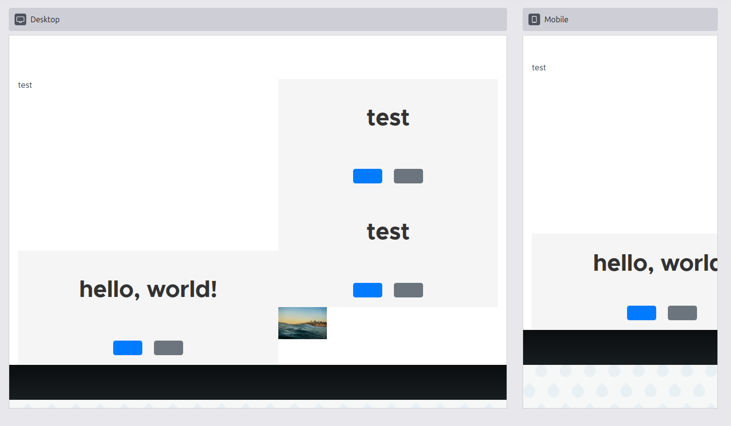
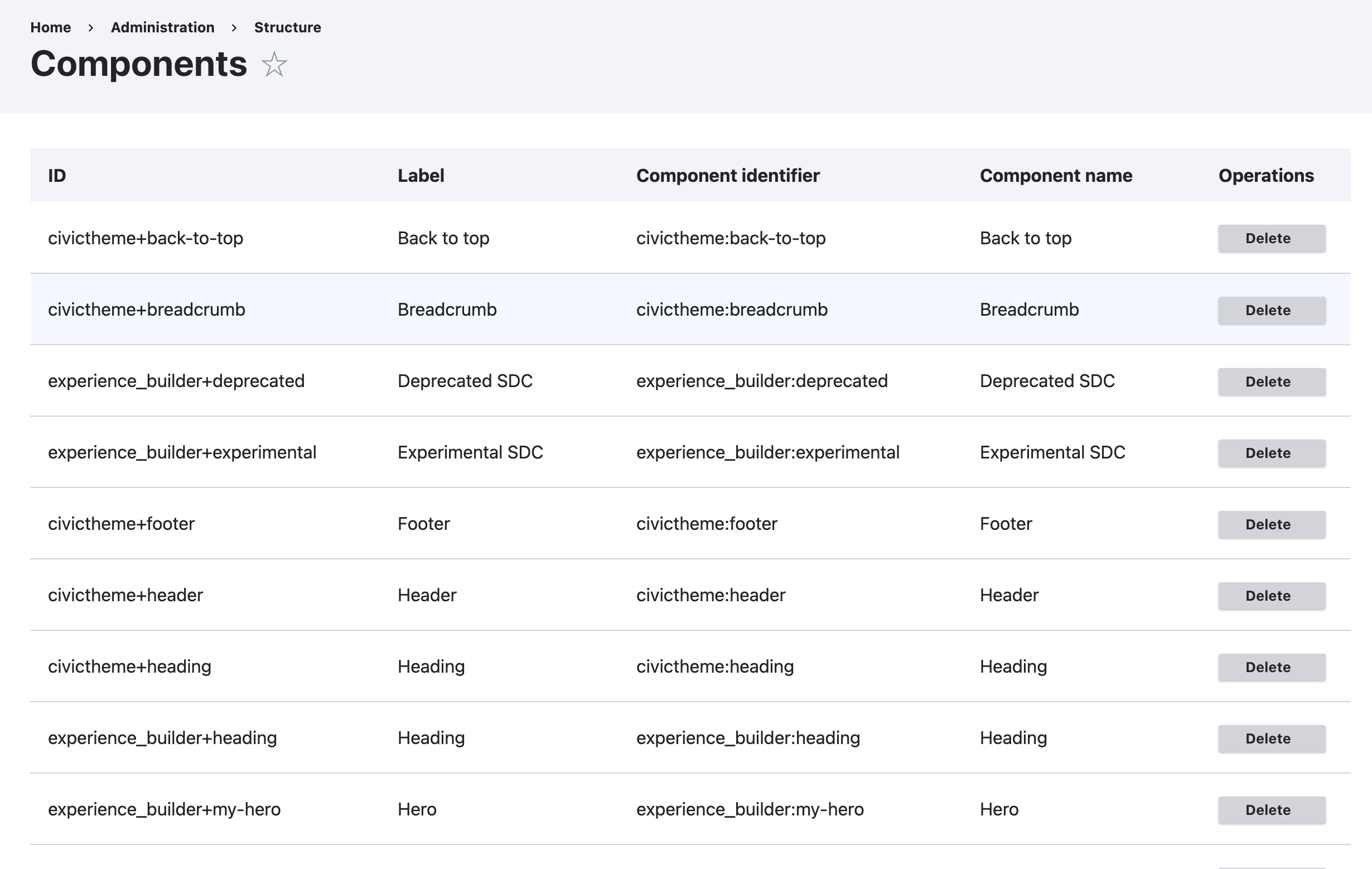
For a huge DX leap forward for both those working on XB itself as well as those working on the Starshot Demo Design System (spearheaded by Kristen Pol): Felix’ MR to auto-create/update Component config entities for all discovered Single-Directory Components (SDCs) landed — if they meet the minimum criteria.
For example, each SDC prop must have a title defined, because otherwise XB would be forced to expose machine names, like I mentioned at the start of last week’s update. So: XB requires SDCs to have rich enough metadata to be able to generate a good UX.
That also allowed Omkar “omkar-pd” Deshpande to remove the awkward-but-necessary-at-the-time add/edit form we’d added months ago. When installing the demo_design_system theme, you’ll see something like:
Issue #3464025, image by me.
Ted helped the back end race ahead of the front end: while we don’t have designs for it yet (nor capacity to build it before DrupalCon if they would suddenly exist), there now is an HTTP API to get a list of viable candidate field properties that are able to correctly populate a particular component prop. These are what in the current XB terminology are called dynamic prop sources 2 3.
The preview in the XB UI has been loading component CSS/JS for a while, but thanks to Dave & Ted it now also loads the default theme’s global CSS/JS.
More accurate previews, including for example the Olivero font stack, background and footer showing up.
Issue #3468106, image by Dave. Small(ish) but noteworthy
- Ted proved via a test that both symmetric and asymmetric translations work correctly in the current data model/field type implementation
- Bálint “balintbrews” Kléri & Ben “bnjmnm” Mullins fixed the component props form showing the wrong values
- Now that component trees started working (since last week), Jesse “jessebaker” Baker discovered that it is not actually possible to drag and drop a nested component :D Harumi “hooroomoo” Jang quickly squashed that bug!
- Felix and I were able to narrow down why images with spaces in the filename were being refused to be rendered by the SDC subsystem: Drupal core’s File entity type stores a file stream wrapper URI like public://cat and dog.jpg and considers that a valid URL … but it’s not! URIs cannot contain spaces — that should be encoded as public://cat%20and%20dog.jpg to be valid.
SDC is right, the >10 year old PrimitiveTypeConstraintValidator is wrong! This is being added to the increasingly long list of low-level bugs in Drupal core that went unnoticed for over a decade, so we worked around it for now. - Utkarsh “utkarsh_33” fixed a bug where the name/label of a component instance was lost.
- Finally, a hilarious one to end with: at some point, we set up the “canvas” to be to 10,000x10,000 pixels. Unfortunately, this means that people trying XB have sometimes gotten lost :D
So Jesse reduced it to a mere 3500x3500 pixels, for now that’s sufficient, later we’ll compute this dynamically.
Week 15 was August 19–25, 2024.
-
Yes, that’s the third time I’m linking to docs/data-model.md. It’s that important! ↩︎
-
Dynamic Prop Sources are similar to Drupal’s tokens, but are more precise, and support more than only strings, because SDC props often require more complex shapes than just strings. ↩︎
-
This is the shape matching from ~3 months ago made available to the client side. ↩︎
The Drop Times: Starshot at Barcelona: 10 Sessions on Drupal CMS You Shouldn't Miss
Real Python: Python News Roundup: September 2024
As the autumn leaves start to fall, signaling the transition to cooler weather, the Python community has warmed up to a series of noteworthy developments. Last month, a new maintenance release of Python 3.12.5 was introduced, reinforcing the language’s ongoing commitment to stability and security.
On a parallel note, Python continues its reign as the top programming language according to IEEE Spectrum’s annual rankings. This sentiment is echoed by the Python Developers Survey 2023 results, which reveal intriguing trends and preferences within the community.
Looking ahead, PEP 750 has proposed the addition of tag strings in Python 3.14, inspired by JavaScript’s tagged template literals. This feature aims to enhance string processing, offering developers more control and expressiveness.
Furthermore, EuroSciPy 2024 recently concluded in Poland after successfully fostering cross-disciplinary collaboration and learning. The event featured insightful talks and hands-on tutorials, spotlighting innovative tools and libraries that are advancing scientific computing with Python.
Let’s dive into the most significant Python news from the past month!
Python 3.12.5 ReleasedEarly last month, Python 3.12.5 was released as the fifth maintenance update for the 3.12 series. Since the previous patch update in June, this release packs over 250 bug fixes, performance improvements, and documentation enhancements.
Here are the most important highlights:
- Standard Library: Many modules in the standard library received crucial updates, such as fixes for crashes in ssl when the main interpreter restarts, and various corrections for error-handling mechanisms.
- Core Python: The core Python runtime has several enhancements, including improvements to dictionary watchers, error messages, and fixes for edge-case crashes involving f-strings and multithreading.
- Security: Key security improvements include the addition of missing audit events for interactive Python use and socket connection authentication within a fallback implementation on platforms such as Windows, where Unix inter-process communication is unavailable.
- Tests: New test cases have been added and bug fixes have been applied to prevent random memory leaks during testing.
- Documentation: Python documentation has been updated to remove discrepancies and clarify edge cases in multithreaded queues.
Additionally, Python 3.12.5 comes equipped with pip 24.2 by default, bringing a slew of significant improvements to enhance security, efficiency, and functionality. One of the most notable upgrades is that pip now defaults to using system certificates, bolstering security measures when managing and installing third-party packages.
Read the full article at https://realpython.com/python-news-september-2024/ »[ Improve Your Python With 🐍 Python Tricks 💌 – Get a short & sweet Python Trick delivered to your inbox every couple of days. >> Click here to learn more and see examples ]
PyCharm: How to Use Jupyter Notebooks in PyCharm
PyCharm is one of the most well-known data science tools, offering excellent out-of-the-box support for Python, SQL, and other languages. PyCharm also provides integrations for Databricks, Hugging Face and many other important tools. All these features allow you to write good code and work with your data and projects faster.
PyCharm Professional’s support for Jupyter notebooks combines the interactive nature of Jupyter notebooks with PyCharm’s superior code quality and data-related features. This blog post will explore how PyCharm’s Jupyter support can significantly boost your productivity.
Watch this video to get a comprehensive overview of using Jupyter notebooks in PyCharm and learn how you can speed up your data workflows.
Speed up data analysis Get acquainted with your dataWhen you start working on your project, it is extremely important to understand what data you have, including information about the size of your dataset, any problems with it, and its patterns. For this purpose, your pandas and Polars DataFrames can be rendered in Jupyter outputs in Excel-like tables. The tables are fully interactive, so you can easily sort one or multiple columns and browse and view your data, you can choose how many rows will be shown in a table and perform many other operations.
The table also provides some important information for example:
- You can find the the size of a table in its header.
- You can find the data type symbols in the column headers.
- You can also use JetBrains AI Assistant to get information about your DataFrame by clicking on the icon.
After getting acquainted with your data, you need to clean it. This an important step, but it is also extremely time consuming because there are all sorts of problems you could find, including missing values, outliers, inconsistencies in data types, and so on. Indeed, according to the State of Developer Ecosystem 2023 report, nearly 50% of Data Professionals dedicate 30% of their time or more to data preparation. Fortunately, PyCharm offers a variety of features that streamline the data-cleaning process.
Some insights are already available in the column headers.
First, we can easily spot the amount of missing data for each column because it is highlighted in red. Also, we may be able to see at a glance whether some of our columns have outliers. For example, in the bath column, the maximum value is significantly higher than the ninety-fifth percentile. Therefore, we can expect that this column has at least one outlier and requires our attention.
Additionally, you might suspect there’s an issue with the data if the data type does not match the expected one. For example, the header of the total_sqft column below is marked with the symbol, which in PyCharm indicates that the column contains the Object data type. The most appropriate data type for a column like total_sqft would likely be float or integer, however, so we may expect there to be inconsistencies in the data types within the column, which could affect data processing and analysis. After sorting, we notice one possible reason for the discrepancy: the use of text in data and ranges instead of numerical values.
So, our suspicion that the column had data-type inconsistencies was proven correct. As this example shows, small details in the table header can provide important information about your data and alert you to issues that need to be addressed, so it’s always worth checking.You can also use no-code visualizations to gather information about whether your data needs to be cleaned. Simply click on the icon in the top-left corner of the table. There are many available visualization options, including histograms, that can be used to see where the peaks of the distribution are, whether the distribution is skewed or symmetrical, and whether there are any outliers.
Of course, you can use code to gather information about your dataset and fix any problems you’ve identified. However, the mentioned low-code features often provide valuable insights about your data and can help you work with it much faster.
Code faster Code completion and quick documentationA significant portion of a data professional’s job involves writing code. Fortunately, PyCharm is well known for its features that allow you to write code significantly faster. For example, local ML-powered full line code completion can provide suggestions for entire lines of code.
Another useful feature is quick documentation, which appears when you hover the cursor over your code. This allows you to gather information about functions and other code elements without having to leave the IDE.
RefactoringsOf course, working with code and data is an interactive process, and you may often decide to make some changes in your code – for example, to rename a variable. Going through the whole file or, in some cases, the entire project, would be cumbersome and time consuming. We can use PyCharm’s refactoring capabilities to rename a variable, introduce a constant, and make many other changes in your code. For example, in this case, I want to rename the DataFrame to make it shorter. I simply use the the Rename refactoring to make the necessary changes.
PyCharm offers a vast number of different refactoring options. To dive deeper into this functionality, watch this video.
Fix problemsIt is practically impossible to write code without there being any mistakes or typos. PyCharm has a vast array of features that allow you to spot and address issues faster. You will notice the Inspection widget in the top-right corner if it finds any problems.
For example, I forgot to import a library in my project and made several typos in the doc so let’s take a look how PyCharm can help here.
First of all, the problem with the library import:
Additionally, with Jupyter traceback, you can see the line where the error occurred and get a link to the code. This makes the bug-fixing process much easier. Here, I have a typo in line 3. I can easily navigate to it by clicking on the blue text.
Additionally if you would like to get more information and suggestion how to fix the problem, you can use JetBrains AI Assistant by clicking on Explain with AI.
Of course, that is just the tip of the iceberg. We recommend reading the documentation to better understand all the features PyCharm offers to help you maintain code quality.
Navigate easilyFor the majority of cases, data science work involves a lot of experimentation, with the journey from start to finish rarely resembling a straight line.
During this experimentation process, you have to go back and forth between different parts of your project and between cells in order to find the best solution for a given problem. Therefore, it is essential for you to be able to navigate smoothly through your project and files. Let’s take a look at how PyCharm can help in this respect.
First of all, you can use the classic CMD+F (Mac) or CTRL+F (Windows) shortcut for searching in your notebook. This basic search functionality offers some additional filters like Match Case or Regex.
You can use Markdown cells to structure the document and navigate it easily.
If you would like to highlight some cells so you can come back to them later, you can mark them with #TODO or #FIXME, and they will be made available for you to dissect in a dedicated window.
Or you can use tags to highlight some cells so you’ll be able to spot them more easily.
In some cases, you may need to see the most recently executed cell; in this case, you can simply use the Go To option.
Save your workBecause teamwork is essential for data professionals, you need tooling that makes sharing the results of your work easy. One popular solution is Git, which PyCharm supports with features like notebook versioning and version comparison using the Diff view. You can find an in-depth overview of the functionality in this tutorial.
Another useful feature is Local History, which automatically saves your progress and allows you to revert to previous steps with just a few clicks.
Use the full power of AI AssistantJetBrains AI Assistant helps you automate repetitive tasks, optimize your code, and enhance your productivity. In Jupyter notebooks, it also offers several unique features in addition to those that are available in any JetBrains tool.
Click the icon to get insights regarding your data. You can also ask additional questions regarding the dataset or ask AI Assistant to do something – for example, “write some code that solves the missing data problem”.
AI data visualizationPressing the icon will suggest some useful visualizations for your data. AI Assistant will generate the proper code in the chat section for your data.
AI cellAI Assistant can create a cell based on a prompt. You can simply ask it to create a visualization or do something else with your code or data, and it will generate the code that you requested.
DebuggerPyCharm offers advanced debugging capabilities to enhance your experience in Jupyter notebooks. The integrated Jupyter debugger allows you to set breakpoints, inspect variables, and evaluate expressions directly within your notebooks. This powerful tool helps you step through your code cell by cell, making it easier to identify and fix issues as they arise. Read our blog post on how you can debug a Jupyter notebook in PyCharm for a real-life example.
Get started with PyCharm ProfessionalPyCharm’s Jupyter support enhances your data science workflows by combining the interactive aspects of Jupyter notebooks with advanced IDE features. It accelerates data analysis with interactive tables and AI assistance, improves coding efficiency with code completion and refactoring, and simplifies error detection and navigation. PyCharm’s seamless Git integration and powerful debugging tools further boost productivity, making it essential for data professionals.
Download PyCharm Professional to try it out for yourself! Get an extended trial today and experience the difference PyCharm Professional can make in your data science endeavors.Use the promo code “PyCharmNotebooks” at checkout to activate your free 60-day subscription to PyCharm Professional. The free subscription is available for individual users only.
Activate your 60-day trialExplore our official documentation to fully unlock PyCharm’s potential for your projects.
Mike Driscoll: Adding Terminal Effects with Python
The Python programming language has thousands of wonderful third-party packages available on the Python Package Index. One of those packages is TerminalTextEffects (TTE), a terminal visual effects engine.
Here are the features that TerminalTextEffects provides, according to their documentation:
- Xterm 256 / RGB hex color support
- Complex character movement via Paths, Waypoints, and motion easing, with support for quadratic/cubic bezier curves.
- Complex animations via Scenes with symbol/color changes, layers, easing, and Path synced progression.
- Variable stop/step color gradient generation.
- Path/Scene state event handling changes with custom callback support and many pre-defined actions.
- Effect customization exposed through a typed effect configuration dataclass that is automatically handled as CLI arguments.
- Runs inline, preserving terminal state and workflow.
Note: This package may be somewhat slow in Windows Terminal, but it should work fine in other terminals.
Let’s spend a few moments learning how to use this neat package
InstallationThe first step to using any new package is to install it. You can use pip or pipx to install TerminalTextEffects. Here is the typical command you would run in your terminal:
python -m pip install terminaltexteffectsNow that you have TerminalTextEffects installed, you can start using it!
UsageLet’s look at how you can use TerminalTextEffects to make your text look neat in the terminal. Open up your favorite Python IDE and create a new file file with the following contents:
from terminaltexteffects.effects.effect_slide import Slide text = ("PYTHON" * 10 + "\n") * 10 effect = Slide(text) effect.effect_config.merge = True with effect.terminal_output() as terminal: for frame in effect: terminal.print(frame)This code will cause the string, “Python” to appear one hundred times with ten strings concatenated and ten rows. You use a Slide effect to make the text slide into view. TerminalTextEffects will also style the text too.
When you run this code, you should see something like the following:
TerminalTextEffects has many different built-in effects that you can use as well. For example, you can use Beams to make the output even more interesting. For this example, you will use the Zen of Python text along with the Beams effects:
from terminaltexteffects.effects.effect_beams import Beams TEXT = """ The Zen of Python, by Tim Peters Beautiful is better than ugly. Explicit is better than implicit. Simple is better than complex. Complex is better than complicated. Flat is better than nested. Sparse is better than dense. Readability counts. Special cases aren't special enough to break the rules. Although practicality beats purity. Errors should never pass silently. Unless explicitly silenced. In the face of ambiguity, refuse the temptation to guess. There should be one-- and preferably only one --obvious way to do it. Although that way may not be obvious at first unless you're Dutch. Now is better than never. Although never is often better than *right* now. If the implementation is hard to explain, it's a bad idea. If the implementation is easy to explain, it may be a good idea. Namespaces are one honking great idea -- let's do more of those! """ effect = Beams(TEXT) with effect.terminal_output() as terminal: for frame in effect: terminal.print(frame)Now try running this code. You should see something like this:
That looks pretty neat! You can see a whole bunch of other effects you can apply on the package’s Showroom page.
Wrapping UpTerminalTextEffects provides lots of neat ways to jazz up your text-based user interfaces with Python. According to the documentation, you should be able to use TerminalTextEffects in other TUI libraries, such as Textual or Asciimatics, although it doesn’t specifically state how to do that. Even if you do not do that, you could use TerminalTextEffects with the Rich package to create a really interesting application in your terminal.
Links
The post Adding Terminal Effects with Python appeared first on Mouse Vs Python.
Pages
Recent Publications
- Managing Hidden Dependencies in OO Software: a Study Based on Open Source Projects
- Open Source Communities as Liminal Ecosystems
- Investigating developers' email discussions during decision-making in Python language evolution
- Developers, Quality Control and Download Volume in Open Source Software (OSS) Projects