
Feeds
Making a Difference
How to contribute and jump start your career in Free Software with the KDE Community
With Aleix Pol, KDE e.V. President and core contributing developer of (among other many things) KDE Connect, Plasma, Discover and KAlgebra.
Bits from Debian: DebConf24 closes in Busan and DebConf25 dates announced
On Saturday 3 August 2024, the annual Debian Developers and Contributors Conference came to a close.
Over 339 attendees representing 48 countries from around the world came together for a combined 108 events made up of Talks, Discussions, Birds of a Feather (BoF) gatherings, workshops, and activities in support of furthering our distribution and free software (25 patches submitted to the Linux kernel), learning from our mentors and peers, building our community, and having a bit of fun.
The conference was preceded by the annual DebCamp hacking session held July 21st through July 27th where Debian Developers and Contributors convened to focus on their Individual Debian related projects or work in team sprints geared toward in-person collaboration in developing Debian.
This year featured a BootCamp that was held for newcomers with a GPG Workshop and a focus on Introduction to creating .deb files (Debian packaging) staged by a team of dedicated mentors who shared hands-on experience in Debian and offered a deeper understanding of how to work in and contribute to the community.
The actual Debian Developers Conference started on Sunday July 28 2024.
In addition to the traditional 'Bits from the DPL' talk, the continuous key-signing party, lightning talks and the announcement of next year's DebConf25, there were several update sessions shared by internal projects and teams.
Many of the hosted discussion sessions were presented by our technical core teams with the usual and useful meet the Technical Committee and the ftpteam and a set of BoFs about packaging policy and Debian infrastructure, including talk about APT and Debian Installer. Internationalization and localization have been subject of several talks. The Python, Perl, Ruby, and Go programming language teams, as well as Med team, also shared updates on their work and efforts.
More than fifteen BoFs and talks about community, diversity and local outreach highlighted the work of various team involved in the social aspect of our community. This year again, Debian Brazil shared strategy and action to attract and retain new contributors and members and opportunities both in Debian and F/OSS.
The schedule was updated each day with planned and ad-hoc activities introduced by attendees over the course of the conference. Several traditional activities were performed: a job fair, a poetry performance, the traditional Cheese and Wine party, the group photos and the Day Trips.
For those who were not able to attend, most of the talks and sessions were videoed for live room streams with the recorded videos made available through a link in their summary in the schedule. Almost all of the sessions facilitated remote participation via IRC messaging apps or online collaborative text documents which allowed remote attendees to 'be in the room' to ask questions or share comments with the speaker or assembled audience.
DebConf24 saw over 6.8 TiB of data streamed, 91.25 hours of scheduled talks, 20 network access points, 1.6 km fibers (1 broken fiber...) and 2.2 km UTP deployed, more than 20 country Geoip viewers, 354 T-shirts, 3 day trips, and up to 200 meals planned per day.
All of these events, activities, conversations, and streams coupled with our love, interest, and participation in Debian and F/OSS certainly made this conference an overall success both here in Busan, South Korea and On-line around the world.
The DebConf24 website will remain active for archival purposes and will continue to offer links to the presentations and videos of talks and events.
Next year, DebConf25 will be held in Brest, France, from Monday, July 7 to Monday, July 21, 2025. As tradition follows before the next DebConf the local organizers in France will start the conference activities with DebCamp with particular focus on individual and team work towards improving the distribution.
DebConf is committed to a safe and welcome environment for all participants. See the web page about the Code of Conduct in DebConf24 website for more details on this.
Debian thanks the commitment of numerous sponsors to support DebConf24, particularly our Platinum Sponsors: Infomaniak, Proxmox, and Wind River.
We also wish to thank our Video and Infrastructure teams, the DebConf24 and DebConf committees, our host nation of South Korea, and each and every person who helped contribute to this event and to Debian overall.
Thank you all for your work in helping Debian continue to be "The Universal Operating System".
See you next year!
About DebianThe Debian Project was founded in 1993 by Ian Murdock to be a truly free community project. Since then the project has grown to be one of the largest and most influential open source projects. Thousands of volunteers from all over the world work together to create and maintain Debian software. Available in 70 languages, and supporting a huge range of computer types, Debian calls itself the universal operating system.
About DebConfDebConf is the Debian Project's developer conference. In addition to a full schedule of technical, social and policy talks, DebConf provides an opportunity for developers, contributors and other interested people to meet in person and work together more closely. It has taken place annually since 2000 in locations as varied as Scotland, Argentina, Bosnia and Herzegovina, and India. More information about DebConf is available from https://debconf.org/.
About InfomaniakInfomaniak is an independent cloud service provider recognized throughout Europe for its commitment to privacy, the local economy and the environment. Recording growth of 18% in 2023, the company is developing a suite of online collaborative tools and cloud hosting, streaming, marketing and events solutions. Infomaniak uses exclusively renewable energy, builds its own data centers and develops its solutions in Switzerland, without relocating. The company powers the website of the Belgian radio and TV service (RTBF) and provides streaming for more than 3,000 TV and radio stations in Europe.
About ProxmoxProxmox provides powerful and user-friendly Open Source server software. Enterprises of all sizes and industries use Proxmox solutions to deploy efficient and simplified IT infrastructures, minimize total cost of ownership, and avoid vendor lock-in. Proxmox also offers commercial support, training services, and an extensive partner ecosystem to ensure business continuity for its customers. Proxmox Server Solutions GmbH was established in 2005 and is headquartered in Vienna, Austria. Proxmox builds its product offerings on top of the Debian operating system.
About Wind RiverWind River For nearly 20 years, Wind River has led in commercial Open Source Linux solutions for mission-critical enterprise edge computing. With expertise across aerospace, automotive, industrial, telecom, and more, the company is committed to Open Source through initiatives like eLxr, Yocto, Zephyr, and StarlingX.
Contact InformationFor further information, please visit the DebConf24 web page at https://debconf24.debconf.org/ or send mail to press@debian.org.
The Drop Times: Which CMS Powers the Top US University Websites? A Comprehensive Analysis
Thorsten Alteholz: My Debian Activities in July 2024
This month I accepted 502 and rejected 40 packages. The overall number of packages that got accepted was 515.
In case you want to upload dozens of packages, it would be nice to give some heads-up before. It is kind of a shock to see a full NEW queue in the morning, though it was much shorter in the evening before.
Debian LTSThis was my hundred-twenty-first month that I did some work for the Debian LTS initiative, started by Raphael Hertzog at Freexian.
- [#1074439] bookworm-pu: cups 2.4.2-3+deb12u7 has been marked for accept
This month I finished the new version of tiff for Bullseye (and Bookworm). The upload will follow, when Bullseye has been handed over to the LTS team in August.
Last but not least I attended the monthly LTS/ELTS meeting.
Debian ELTSThis month was the seventy-second ELTS month. During my allocated time I uploaded or worked on:
- [ELA-1126-1-1]exim4 security update for one CVE. This was the delayed ELA I mentioned in my last report.
- [ELA-1144-1-1]exim4 security update for one CVE to fix parsing of multiline RFC 2231 header filenames in Stretch and Buster. Jessie was not affected by this issue.
- Uploaded new versions of tiff for Jessie and Stretch that got stuck in the autopkgtests.
For whatever reason, I had trouble with the CI again. The new tiff package wanted to run the autopkgtest of cups but never did it. So the corresponding ELA will appear only in August.
I also continued to work on an update for libvirt. There really is a reason why some packages don’t get much attention. Nevertheless someone has to take care of them. I also did a week of FD and attended the LTS/ELTS meeting.
Debian PrintingThis month I uploaded …
- … lprint to fix a /usr-move issue
- … magicfilter to fix a gcc14 issue
This work is generously funded by Freexian!
Debian AstroThis month I uploaded a new upstream or bugfix version of:
- … libplayerone to fix a /usr-move issue
- … libsbig to fix a /usr-move issue
- … libfli to fix a /usr-move issue
- … libfishcamp to fix a /usr-move issue
This month I uploaded new upstream or bugfix versions of:
- … pyicloud to update dependencies
This month I uploaded …
- … libsmpp34 to fix a gcc14 issue
The following packages have been prepared by the GSoC student Nathan:
- … osmo-trx
- … osmo-pcu
- … libosmocore (another new upstream version)
This month I uploaded new upstream or bugfix versions of:
- … meep to add autopkgtest
- … meep-mpi-default to add autopkgtest
- … meep-openmpi to add autopkgtest
- … a56 to fix a gcc14 issue (patch provided by Ben)
- … setserial to fix a gcc14 issue
- … scheme48 to fix a gcc14 issue
- … bottlerocket to fix a gcc14 issue
- … uucp to fix a gcc14 issue
Russell Coker: PineTime Status
Since my last blog post about the PineTime [1] I haven’t done anything exciting with it. I’ve been wearing it every day and it’s working reasonably well for me. It’s been working better since I changed to a Samsung Galaxy Note 9 as my main phone [2], so it seems that the Huawei Mate 10 Pro has some issues with Bluetooth that were making it unreliable.
A relative also has one which is working well for them but which had some problems, I only discovered that holding the button down for a long time (longer than usual for device reset) makes a PineTime reboot because of their issues. I also once had their device get into a bad state where the only thing I could do was flash a newer firmware which fortunately fixed the problem.
My latest issue is the battery life. Recently it has been taking ages to get above about 90% charge when charging and the time taken to go down to ~70% when I charge it seems to be decreasing. Yesterday it suddenly went to 13% after being 73% the previous night. Then it stayed at 13% all day. It seems quite inaccurate. But also it doesn’t seem to be lasting as long as before.
Generally it seems to me that Pine64 products are almost great. I won’t rule out the possibility of a newer firmware for the PineTime alleviating the battery issues (or at least reporting the status accurately) and making Bluetooth connectivity more reliable (even on older phones). For the PinePhonePro an update to Mobian could reduce power wasting from user space (there’s an issue that I have reported in Plasma Mobile but no-one is interested on working on this before KDE 6), and a kernel update could improve things. But I don’t think there’s a possibility of it ever having the battery last a day while polling Matrix and Jabber servers which is something that every Android phone can do without problems.
- [1] https://etbe.coker.com.au/2023/10/21/more-about-pinetime/
- [2] https://etbe.coker.com.au/2024/07/01/volte-australia/
Related posts:
- Bluetooth Versions and PineTime I’ve done some tests with the PineTime [1] on different...
- More About the PineTime Since my initial review of the PineTime 10 days ago...
- The PineTime I have just got a PineTime smart watch [1] from...
This week in KDE: SVG Breeze cursors and more thumbnails
First up is something cool: support for SVG-based cursor themes! This allows compatible themes to always display beautiful sharp cursors at any size, and has already been rolled out for the Breeze Light and Breeze Dark cursor themes. It does not use the Hyprcursor system, and we have not yet upstreamed it to be a different cross-desktop spec. However, we are considering doing so in the near future. This work was done by Jin Liu and Vlad Zahorodnii, and lands in Plasma 6.2.0.
On the subject of cross-desktop specs, KDE apps now does support the cross-desktop thumbnailer spec, meaning that any of these thumbnailers already on the system will now instantly start working! One of the most notable examples would be the STL file thumbnailer, which will be a boon for anyone working with 3D models or 3D printers. This work was done by Akseli Lahtinen and lands in KDE Frameworks 6.6. You can read about it more in this blog post.
That isn’t all, though…
More Notable New FeaturesElisa now shows the total duration of the songs from the playlist in its footer (Karl Hoffman, Elisa 24.12.0. Link):
Plasma now lets you escape from the tyranny of time by hiding the clocks on the login and lock screens entirely (Someone going by the pseudonym “Be Ing”, Plasma 6.2.0. Link)
Plasma’s Pager widget now lets you turn off window outlines if you’d prefer a cleaner display of only the virtual desktops (Christian Muehlhaeuser, Plasma 6.2.0. Link)
The Breeze Light and Breeze Dark Plasma styles (not color schemes, Plasma styles) now respect your systemwide accent color too. In particular, this makes the built-in Breeze Twilight Global Theme fully accent-color-aware (Niccolò Venerandi, Plasma 6.2.0. Link):
Notable UI ImprovementsElisa now remembers window maximization state and prior window geometry across launches as expected (me: Nate Graham, Elisa 24.08.0. Link)
Filelight now remembers its window size (and position, on X11) across launches (me: Nate Graham, Filelight, 24.12.0. Link)
When using background blur e.g. in apps like Konsole, there’s no longer a blurry sharp corner poking out of the rounded titlebar corners (Xaver Hugl, Plasma 6.2.0. Link)
Notable Bug FixesFixed a silly bug that caused System Settings’ Display & Monitor page to be unable to show auto-rotate settings the first time it was opened (Marco Martin, Plasma 6.1.4. Link)
When you click on column headers in System Monitor to sort a table by a different column, they’re now ordered top-to-bottom as expected (Arjen Hiemstra, Plasma 6.1.5. Link)
Worked around a quirk in VLC, with the net result that standard MPRIS-compatible play/pause controls (e.g. via global shortcut, dedicated keyboard keys, or the Media Player widget) work again (Fushan Wen, Plasma 6.1.5. Link)
Worked around a Qt bug that caused widgets in Plasma’s Widget Explorer to overlap after clearing the search field text with animations globally disabled (me: Nate Graham and Noah Davis, Plasma 6.1.5. Link)
Fixed a bug that caused the “copy time/date to clipboard” feature of Plasma’s Digital Clock widget to not work on Wayland. This should also more generally help with clipboard issues where the source window disappears after content is copied (David Redondo, Plasma 6.2.0. Link)
The “Small font” setting on System Settings’ Fonts page now works again, because we fixed a subtle Plasma 6 porting error that broke it (Marco Martin, Frameworks 6.6. Link)
Other bug information of note:
- 3 Very high priority Plasma bugs (up from 1 last week). Current list of bugs
- 31 15-minute Plasma bugs (same as last week). Current list of bugs
- 94 KDE bugs of all kinds fixed over the last week. Full list of bugs
Fixed an issue that caused noticeable frame drop when using certain hybrid Intel+NVIDIA GPU setups (Xaver Hugl, Plasma 6.1.4. Link)
You can now drag-and-drop stuff to an Plasma panel in auto-hide mode on Wayland; it un-hides as needed, just like it does on X11 (Yifan Zhu, Plasma 6.1.5. Link)
Changing the language on System Settings Region & Language page is now more reliable, accounting for cases where distros might not set things up quite right themselves (Han Young, Plasma 6.1.5. Link)
Improved the speed and performance of Discover’s search feature (Aleix Pol Gonzalez, Plasma 6.1.5. Link)
Improved system performance when using ICC color profiles (Xaver Hugl, Plasma 6.2.0. Link)
Video players are now more likely to be to able to trigger KWin’s direct scan-out feature, saving power and system resources (Xaver Hugl, Plasma 6.2.0. Link)
Made Plasma’s Global Menu feature work more reliably on Wayland with exported menus from Electron apps like VSCode (David Redondo, Plasma 6.2.0. Link)
…And Everything ElseThis blog only covers the tip of the iceberg! If you’re hungry for more, check out https://planet.kde.org, where you can find more news from other KDE contributors.
How You Can HelpOtherwise, visit https://community.kde.org/Get_Involved to discover other ways to be part of a project that really matters. Each contributor makes a huge difference in KDE; you are not a number or a cog in a machine! You don’t have to already be a programmer, either. I wasn’t when I got started. Try it, you’ll like it! We don’t bite! Or consider donating instead! That helps too.
Carl Trachte: Embedding an SVG in a graphviz Generated SVG and More DAG Hamilton
Last time I used a previous post's DAG Hamilton graphviz output to generate a series of functionally highlighted DAG Hamilton workflow graphs. The SVG (scalable vector graphics) versions of these graphs will serve as the input for this post.
I was dissatisfied with the quality of the PNG output, or at least how it rendered, fuzzy and illegible. My thought was that an SVG presentation would provide a more crisp, scalable (hence the name SVG) view of each graph.
Where I ran into problems was the embedded logos. Applications like PowerPoint allowed the inclusion of the logos as SGV "images" within the SVG "image" in PowerPoint, but did not render them; blank spaces remained.
So I set out to embed the SVG of the logos inline as elements within the final SVG file; it turned into quite the journey . . .
So SVG is really just XML, right? No, it is XML; it's just not just XML. There are XML tags and what is inside those tags can contain multiple SVG characteristics, all in their own syntax, most listed as quoted text.
At this point finding a library that allows for programmatic manipulation of SGV by tag or reviewing some open source browser source code may have helped. I did not do either of those things (a brief internet search yielded Python libraries, but they seemed focused more on conversion to and from SVG and other image formats) and set out on my own.
Like most people, I have played with Inkscape and converted images to SVG format. I even blogged about having done this with POVRay rendered pysanky eggs back in the day. Using something with software written by people way smarter than you and actually understanding it are two entirely different animals.
To make matters worse . . . I cannot actually display the SVG images or inline them here on Blogger. Smaller SVG snippets seem to work, but an entire graph with SVG logos is either too much or I am doing something wrong. Another (blurry) PNG example of the output will have to do.
Important concepts with links:
1) viewBox, scale, dimensions - Soueiden (classic, kind of the standard as far as I can tell):
https://www.sarasoueidan.com/blog/mimic-relative-positioning-in-svg/
2) the four quadrants of svg space (but you only see the lower right):
http://dh.obdurodon.org/coordinate-tutorial.xhtml
3) use x, y positioning to place embedded SVG rather than viewBox coordinates:
I have lost the link, but whoever suggested this, thank you.
4) (no link) Allow graphviz to do as much work as possible before editing any svg. For instance, when bolding edges of the graph in SVG, the edges will invariably overlap the nodes. This looks ugly. graphviz handles all that and it is far far simpler than trying to do it on your own.
5) bezier curves - nothing in this post about them, but they were part of my real introduction to SVG, and the most fun part. Recommend.
https://javascript.info/bezier-curve#de-casteljau-s-algorithm
Methodology for putting SVG logos inside the SVG document (not necessarily in order):
1) scale the embedded SVGs with the "width" and "height" attributes (SVG). I made mine proportional relative to the original SVGs' dimensions.
2) Calculate where the SVGs are supposed to go within the graphviz generated SVG coordinate space.
graphviz pushes everything into the upper right SVG space quadrant with an SVG "translate" command with 4 units padding. This needs to be taken into account when positioning the SVG elements relative to graphviz' coordinate space. The elements will be using the lower right SVG space quadrant coordinate space.
3) Leverage the positioning and size of the original PNG logos to place your SVG ones, then pop the old logo image elements and "erase" the boxes around them (yes, quite hacky, but effective).
This is a Python blog. Nutshell: I used xml.etree.ElementTree and rudimentary text processing of the SVG specific parts to get this done.
The whole thing got quite unwieldy and I turned once again to DAG Hamilton to help me organize and visualize things. (Blurry) screenshot below:
Wow, it looks like you just collected every piece of information you could about all the dimensions and smashed it all together in the final SVG document at the end.
Yes.
Hey, why is that one node just hanging out at a dead end not doing anything?
I was not getting the whole coordinate thing and needed it for reference.
The code:
# run.py - the DAG Hamilton control file.
"""Hamilton wrapper."""
# https://hamilton.dagworks.io/en/latest/concepts/driver/#recap
import sys
import pprint
from hamilton import driver
import editsvgs as esvg
OUTPUTFILES = {'data_source_highlighted':'data_source_highlighted_final', 'web_scraping_functions_highlighted':'web_scraping_functions_highlighted_final', 'output_functions_highlighted':'output_functions_highlighted_final'}
dr = driver.Builder().with_modules(esvg).build()
dr.display_all_functions('esvg.svg', deduplicate_inputs=True, keep_dot=True, orient='BR')
for keyx in OUTPUTFILES: results = dr.execute(['hamilton_logo_root', 'company_logo_root', 'graph_root', 'doc_attrib', 'hamilton_logo_tree_indices', 'company_logo_tree_indices', 'hamilton_logo_png_attrib', 'company_logo_png_attrib', 'parsed_hamiltonlogo_png_attrib', 'parsed_companylogo_png_attrib', 'biggerdimension', 'dimensionratio', 'parsed_graph_dimensions', 'hamilton_logo_position', 'hamilton_svg_dimensions', 'hamilton_logo_dimensions_orig', 'biggerdimension_company', 'dimensionratio_company', 'company_logo_position', 'company_svg_dimensions', 'company_logo_dimensions_orig', 'final_svg_file'], inputs={'hamiltonlogofile':'hamiltonlogolarge.svg', 'companylogofile':'fauxcompanylogo.svg', 'testfile':keyx + '.svg', 'outputfile':OUTPUTFILES[keyx] + '.svg', 'hamiltonlogopng':'hamiltonlogolarge.png', 'companylogopng':'fauxcompanylogo.png'}) print('\ndoc_attrib =\n') pprint.pprint(results['doc_attrib']) print('\nhamilton_logo_tree_indices =\n') pprint.pprint(results['hamilton_logo_tree_indices']) print('\ncompany_logo_tree_indices =\n') pprint.pprint(results['company_logo_tree_indices']) print('\nhamilton_logo_png_attrib =\n') pprint.pprint(results['hamilton_logo_png_attrib']) print('\nparsed_hamiltonlogo_png_attrib =\n') pprint.pprint(results['parsed_hamiltonlogo_png_attrib']) print('\ncompany_logo_png_attrib =\n') pprint.pprint(results['company_logo_png_attrib']) print('\nparsed_companylogo_png_attrib =\n') pprint.pprint(results['parsed_companylogo_png_attrib']) print('\nbiggerdimension =\n') pprint.pprint(results['biggerdimension']) print('\ndimensionratio =\n') pprint.pprint(results['dimensionratio']) print('\nparsed_graph_dimensions =\n') pprint.pprint(results['parsed_graph_dimensions']) print('\nhamilton_logo_position =\n') pprint.pprint(results['hamilton_logo_position']) print('\nhamilton_svg_dimensions =\n') pprint.pprint(results['hamilton_svg_dimensions']) print('\nhamilton_logo_dimensions_orig =\n') pprint.pprint(results['hamilton_logo_dimensions_orig']) print('\ndimensionratio_company =\n') pprint.pprint(results['dimensionratio_company']) print('\ncompany_logo_position =\n') pprint.pprint(results['company_logo_position']) print('\ncompany_svg_dimensions =\n') pprint.pprint(results['company_svg_dimensions']) print('\ncompany_logo_dimensions_orig =\n') pprint.pprint(results['company_logo_dimensions_orig']) print('\nfinal_svg_file =\n') pprint.pprint(results['final_svg_file'])
# editsvgs.py - DAG Hamilton noun-named functions.
# python 3.12
"""Attempt to position svg logos and editflowchart with svg."""
import os
import pprint
import xml.etree.ElementTree as ET
import itertools
import sys
import copy
import reusedfunctions as rf
# Pop this to get rid of png image.# '{http://www.w3.org/1999/xlink}href': 'hamiltonlogolarge.png'}PNG_ATTRIB_KEY = '{http://www.w3.org/1999/xlink}href'# '{http://www.w3.org/1999/xlink}href': 'fauxcompanylogo.png'}
def hamilton_logo_root(hamiltonlogofile:str) -> ET.Element: """ Get root of ElementTree object for Hamilton logo svg file.
hamiltonlogofile is the svg file with the Hamilton logo. """ print('Getting Hamilton logo svg file root Element . . .') return rf.getroot(hamiltonlogofile)
def company_logo_root(companylogofile:str) -> ET.Element: """ Get root of ElementTree object for company logo svg file.
companylogofile is the svg file with the company logo. """ print('Getting company logo svg file root Element . . .') return rf.getroot(companylogofile)
def graph_root(testfile:str) -> ET.Element: """ Gets root Element of graphviz graph svg.
testfile is the graphviz svg file. """ print('Getting root Element of main graph svg file . . .') return rf.getroot(testfile)
def doc_attrib(graph_root:ET.Element) -> dict: """ Gets graphviz svg document's dimensions and viewBox in a dictionary.
graph_root is the graphviz svg file root Element.
Returns dictionary of xml/svg data for doc. """ print('Getting dimensions and viewBox for main graph svg file . . .') return graph_root.attrib
def hamilton_logo_tree_indices(graph_root:ET.Element, hamiltonlogopng:str) -> tuple: """ Get tree indices (3 deep) for original png Hamilton logo on graph.
graph_root is the root Element of graphviz graph svg.
hamiltonlogopng is the name of the png file referenced in the image link in the svg file (string).
Returns 3 tuple of integers. """ print('Getting ElementTree indices for tree for Hamilton png logo Element . . .') return rf.gettreeindices(graph_root, hamiltonlogopng)
def company_logo_tree_indices(graph_root:ET.Element, companylogopng:str) -> tuple: """ Get tree indices (3 deep) for original png company logo on graph.
graph_root is the root Element of graphviz graph svg.
companylogopng is the name of the png file referenced in the image link in the svg file (string).
Returns 3 tuple of integers. """ print('Getting ElementTree indices for tree for company png logo Element . . .') return rf.gettreeindices(graph_root, companylogopng)
def hamilton_logo_png_attrib(graph_root:ET.Element, hamilton_logo_tree_indices:tuple) -> dict: """ Get attrib dictionary for original Hamilton png file Element in graph svg.
graph_root is the root Element of graphviz graph svg.
hamilton_logo_tree_indices are the lookup indices for the Hamilton logo png Element within the xml tree. """ print('Getting attrib dictionary for original Hamilton png file Element in graph svg . . .') return rf.getpngattrib(graph_root, hamilton_logo_tree_indices)
def company_logo_png_attrib(graph_root:ET.Element, company_logo_tree_indices:tuple) -> dict: """ Get attrib dictionary for original company png file Element in graph svg.
graph_root is the root Element of graphviz graph svg.
company_logo_tree_indices are the lookup indices for the company logo png Element within the xml tree. """ print('Getting attrib dictionary for original company png file Element in graph svg . . .') return rf.getpngattrib(graph_root, company_logo_tree_indices)
def parsed_hamiltonlogo_png_attrib(hamilton_logo_png_attrib:dict) -> dict: """ Work dictionary that has information on former location of png Hamilton logo image in the graphviz svg.
Basically getting svg text values into float format.
Returns new dictionary. """ print('Getting svg text values into float format for Hamilton png Element . . .') return rf.parsepngattrib(hamilton_logo_png_attrib)
def parsed_companylogo_png_attrib(company_logo_png_attrib:dict) -> dict: """ Work dictionary that has information on former location of png company logo image in the graphviz svg.
Basically getting svg text values into float format.
Returns new dictionary. """ print('Getting svg text values into float format for company logo png Element . . .') return rf.parsepngattrib(company_logo_png_attrib)
def biggerdimension(hamilton_logo_root:ET.Element) -> str: """ hamilton_logo_root is the ElementTree Element for the big svg Hamilton logo.
Returns 'Y' if the y dimension is the bigger one, and 'X' if the x one is.
Returns None if there is a key error. """ print('Determining bigger dimension for svg Hamilton logo . . .') return rf.getbiggerdimension(hamilton_logo_root)
def dimensionratio(biggerdimension:str, hamilton_logo_root:ET.Element) -> float: """ biggerdimension is a string, 'X' or 'Y'.
hamilton_logo_root is the ElementTree Element for the big svg Hamilton logo.
Returns ratio of bigger dimension to smaller one (float). """ print('Calculating dimensions ratio for Hamilton logo svg . . .') return rf.getdimensionratio(biggerdimension, hamilton_logo_root)
def parsed_graph_dimensions(graph_root:ET.Element) -> tuple: """ Get translate coordinates from graphviz svg root Element.
Returns two tuple of x, y translation. """ graph0dimensions = graph_root[0].attrib coordstr = graph0dimensions['transform'] coordstr = coordstr[coordstr.index('translate'):] coordstr = coordstr[coordstr.index('(') + 1:-1] vals = [float(x) for x in coordstr.split(' ')] return tuple(vals)
def hamilton_logo_position(parsed_graph_dimensions:tuple, parsed_hamiltonlogo_png_attrib:dict) -> tuple: """ parsed_graph_dimensions is an x, y two tuple.
parsed_hamiltonlogo_png_attrib is a dictionary.
Returns x, y position of Hamilton logo svg graphic as a two tuple. """ print('Getting position of Hamilton logo . . .') return rf.getposition(parsed_graph_dimensions, parsed_hamiltonlogo_png_attrib)
def company_logo_position(parsed_graph_dimensions:tuple, parsed_companylogo_png_attrib:dict) -> tuple: """ parsed_graph_dimensions is an x, y two tuple.
parsed_hamiltonlogo_png_attrib is a dictionary.
Returns x, y position of company logo svg graphic as a two tuple. """ print('Getting position of company logo . . .') # Add 4. x = parsed_companylogo_png_attrib['X'] + parsed_graph_dimensions[0] # Add negative number with big absolute value. # Upper right quadrant translation thing. y = parsed_companylogo_png_attrib['Y'] + parsed_graph_dimensions[1] return x, y
def hamilton_svg_dimensions(parsed_hamiltonlogo_png_attrib:dict, biggerdimension:str, dimensionratio:float) -> tuple: """ Get width and height of svg Hamilton logo within final document.
parsed_hamiltonlogo_png_attrib is the dictionary of numeric values associated with the original image position of the Hamilton png logo within the svg document.
biggerdimension is the 'X' or 'Y' value that indicates which dimension is the larger of the two.
dimensionratio is the ratio of the larger dimension to the smaller one.
Returns x, y two tuple of floats. """ print('Getting size of Hamilton logo in final doc . . .') return rf.getdimensions(parsed_hamiltonlogo_png_attrib, biggerdimension, dimensionratio)
def hamilton_logo_dimensions_orig(hamilton_logo_root:ET.Element) -> tuple: """ hamilton_logo_root is the ElementTree Element for the big svg Hamilton logo.
Returns two tuple of width, height. """ print('Retrieving dimensions of Hamilton logo svg . . .') return rf.getdimensionsorig(hamilton_logo_root)
def final_svg_file(testfile:str, outputfile:str, hamilton_logo_root:ET.Element, hamilton_logo_tree_indices:tuple, hamilton_logo_position:tuple, hamilton_svg_dimensions:tuple, hamilton_logo_dimensions_orig:tuple, company_logo_tree_indices:tuple, parsed_companylogo_png_attrib:dict, company_logo_position:tuple, company_logo_root:ET.Element, company_svg_dimensions:tuple, company_logo_dimensions_orig:tuple, ) -> str: """ Replaces image logos with scaleable svg ones.
testfile is the name of the original svg file.
outputfile is the name of the intended final svg file.
hamilton_logo_root is the elementree root object for the Hamilton logo svg file.
hamilton_logo_tree_indices are nested indices indicating the location of the original Hamilton logo png elementree Element within the input svg document.
hamilton_logo_position - x, y tuple - where to put the svg Hamilton logo within the final svg document.
hamilton_svg_dimensions - x, y tuple - width and height of Hamilton svg logo within the final svg document.
hamilton_logo_dimensions_orig - two tuple of width, height of original svg file Hamilton logo.
company_logo_tree_indices are nested indices indicating the location of the original company logo png elementree Element within the input svg document.
company_logo_position - x, y tuple - where to put the svg company logo within the final svg document.
company_logo_root is the elementree root object for the company logo svg file. company_svg_dimensions - x, y tuple - width and height of company svg logo within the final svg document.
company_logo_dimensions_orig - two tuple of width, height of original svg file company logo.
Returns string filename. """ print('Making changes to svg . . .') hlti = hamilton_logo_tree_indices retval = outputfile tree = ET.parse(testfile) root = tree.getroot() # pop Hamilton png print('Popping original Hamilton png logo . . .') root[hlti[0]][hlti[1]][hlti[2]].attrib.pop(PNG_ATTRIB_KEY) print('Appending Hamilton svg to root Element . . .') root.append(hamilton_logo_root) print('Adjusting viewBox for Hamilton svg . . .') root[-1].attrib['viewBox'] = '0.00 0.00 {0:.3f} {1:.3f}'.format(*hamilton_logo_dimensions_orig) print('Adjusting height and width for Hamilton svg . . .') root[-1].attrib['height'] = str(hamilton_svg_dimensions[1]) root[-1].attrib['width'] = str(hamilton_svg_dimensions[0]) print('Positioning Hamilton logo svg within final svg . . .') root[-1].attrib['x'] = str(hamilton_logo_position[0]) root[-1].attrib['y'] = str(hamilton_logo_position[1]) print('Erasing Hamilton logo bounding box . . .') # After popping png, polygon resides one index unit back. root[hlti[0]][hlti[1]][hlti[2] - 1].attrib['stroke'] = 'none' clti = company_logo_tree_indices # pop company png print('Popping original company png logo . . .') root[clti[0]][clti[1]][clti[2]].attrib.pop(PNG_ATTRIB_KEY) print('Adding company logo svg Element to main svg file . . .') root.append(company_logo_root) print('Adjusting viewBox for company svg . . .') root[-1].attrib['viewBox'] = '0.00 0.00 {0:.3f} {1:.3f}'.format(*company_logo_dimensions_orig) print('Adjusting height and width for company svg . . .') root[-1].attrib['height'] = str(company_svg_dimensions[1]) root[-1].attrib['width'] = str(company_svg_dimensions[0]) print('Moving company logo svg to the correct position in the display . . .') # Had to adjust 15 units to get it out of the way of the legend. root[-1].attrib['x'] = str(company_logo_position[0] - 15) root[-1].attrib['y'] = str(company_logo_position[1]) print('Erasing company logo bounding box . . .') # After popping png, polygon resides one index unit back. root[clti[0]][clti[1]][clti[2] - 1].attrib['stroke'] = 'none' print('Writing new svg . . .') tree.write(retval) return retval
def biggerdimension_company(company_logo_root:ET.Element) -> str: """ company_logo_root is the ElementTree Element for the big svg company logo.
Returns 'Y' if the y dimension is the bigger one, and 'X' if the x one is. """ print('Determining bigger dimension for svg company logo . . .') return rf.getbiggerdimension(company_logo_root)
def dimensionratio_company(biggerdimension_company:str, company_logo_root:ET.Element) -> float: """ biggerdimension is a string, 'X' or 'Y'.
company_logo_root is the ElementTree Element for the big svg company logo.
Returns ratio of bigger dimension to smaller one (float). """ print('Calculating dimensions ratio for company logo svg . . .') return rf.getdimensionratio(biggerdimension_company, company_logo_root)
def company_logo_position(parsed_graph_dimensions:tuple, parsed_companylogo_png_attrib:dict) -> tuple: """ parsed_graph_dimensions is an x, y two tuple.
parsed_companylogo_png_attrib is a dictionary.
Returns x, y position of company logo svg graphic as a two tuple. """ print('Getting position of company logo . . .') return rf.getposition(parsed_graph_dimensions, parsed_companylogo_png_attrib)
def company_svg_dimensions(parsed_companylogo_png_attrib:dict, biggerdimension_company:str, dimensionratio_company:float) -> tuple: """ Get width and height of svg company logo within final document.
parsed_companylogo_png_attrib is the dictionary of numeric values associated with the original image position of the company png logo within the svg document.
biggerdimension is the 'X' or 'Y' value that indicates which dimension is the larger of the two.
dimensionratio_company is the ratio of the larger dimension to the smaller one.
Returns x, y two tuple of floats. """ pprint.pprint(parsed_companylogo_png_attrib) print('Getting size of company logo in final doc . . .') return rf.getdimensions(parsed_companylogo_png_attrib, biggerdimension_company, dimensionratio_company)
def company_logo_dimensions_orig(company_logo_root:ET.Element) -> tuple: """ company_logo_root is the ElementTree Element for the big svg company logo.
Returns two tuple of width, height. """ print('Retrieving dimensions of company logo svg . . .') return rf.getdimensionsorig(company_logo_root)
# reusedfunctions.py - utility/helper/main functionality
# at a granular level.
# python 3.12
"""Auxiliary module to Hamilton svg script."""
import itertools
import xml.etree.ElementTree as ET
# Pop this to get rid of png image.# '{http://www.w3.org/1999/xlink}href': 'hamiltonlogolarge.png'}PNG_ATTRIB_KEY = '{http://www.w3.org/1999/xlink}href'
def gettreeindices(graph_root, png): """ Get tree indices (3 deep) for png on graph.
graph_root is the root Element of graphviz graph svg.
png is the name of the png file referenced in the image link in the svg file (string).
Returns 3 tuple of integers. """ countergeneratorx = itertools.count() counterx = next(countergeneratorx) for nodex in graph_root: countergeneratory = itertools.count() countery = next(countergeneratory) for nodey in nodex: countergeneratorz = itertools.count() counterz = next(countergeneratorz) for nodez in nodey: if PNG_ATTRIB_KEY in nodez.attrib: if nodez.attrib[PNG_ATTRIB_KEY] == png: return counterx, countery, counterz counterz = next(countergeneratorz) countery = next(countergeneratory) counterx = next(countergeneratorx)
def getroot(filename): """ Get root of ElementTree object for svg file.
filename is the svg file string. """ return ET.parse(filename).getroot()
def getpngattrib(graph_root, indices): """ Get attrib dictionary for png file Element in graph svg.
graph_root is the root Element of graphviz graph svg.
indices are the lookup indices for the png Element within the xml tree. """ return graph_root[indices[0]][indices[1]][indices[2]].attrib
def parsepngattrib(attrib): """ Work dictionary that has information on location of png image in the graphviz svg.
Basically getting svg text values into float format.
Returns new dictionary. """ retval = {} retval['X'] = float(attrib['x']) retval['Y'] = float(attrib['y']) retval['height'] = float(attrib['height'][:attrib['height'].index('px')]) retval['width'] = float(attrib['width'][:attrib['width'].index('px')]) return retval
def getbiggerdimension(root): """ root is the ElementTree Element for the svg file element to be embedded into the main svg file.
Returns 'Y' if the y dimension is the bigger one, and 'X' if the x one is.
Returns None if there is a key error. """ dimensions = root.attrib try: if float(dimensions['height']) > float(dimensions['width']): return 'Y' else: # X bigger or equal return 'X' except ValueError: pass return None
def getdimensionratio(biggerdimension, root): """ biggerdimension is a string, 'X' or 'Y'.
root is the etree Element for the svg Element that is to be embedded into the final svg file
Returns ratio of bigger dimension to smaller one (float). """ dimensions = root.attrib if biggerdimension == 'Y': return float(dimensions['height']) / float(dimensions['width']) else: return float(dimensions['width']) / float(dimensions['height'])
def getposition(dimensions, attrib): """ dimensions is an x, y two tuple.
attrib is a dictionary.
Returns x, y position of svg graphic as a two tuple. """ # Add 4. x = attrib['X'] + dimensions[0] # Add negative number with big absolute value. # Upper right quadrant translation thing. y = attrib['Y'] + dimensions[1] return x, y
def getdimensions(attrib, biggerdimension, dimensionratio): """ Get width and height of svg within final document.
attrib is the dictionary of numeric values associated with the original image position of the png within the svg document.
biggerdimension is the 'X' or 'Y' value that indicates which dimension is the larger of the two.
dimensionratio is the ratio of the larger dimension to the smaller one.
Returns x, y two tuple of floats. """ if biggerdimension == 'Y': return (attrib['width'], dimensionratio * attrib['width']) else: return (dimensionratio * attrib['height'], attrib['height'])
def getdimensionsorig(root): """ root is the ElementTree Element for the svg Element to be embedded in the main svg file.
Returns two tuple of width, height. """ return float(root.attrib['width']), float(root.attrib['height'])
# OUTPUT (stdout)
Getting Hamilton logo svg file root Element . . .Getting company logo svg file root Element . . .Getting root Element of main graph svg file . . .Getting dimensions and viewBox for main graph svg file . . .Getting ElementTree indices for tree for Hamilton png logo Element . . .Getting ElementTree indices for tree for png Element . . .Getting ElementTree indices for tree for company png logo Element . . .Getting ElementTree indices for tree for png Element . . .Getting attrib dictionary for original Hamilton png file Element in graph svg . . .Getting attrib dictionary for original company png file Element in graph svg . . .Getting svg text values into float format for Hamilton png Element . . .Getting svg text values into float format for company logo png Element . . .Determining bigger dimension for svg Hamilton logo . . .Calculating dimensions ratio for Hamilton logo svg . . .Getting position of Hamilton logo . . .Getting size of Hamilton logo in final doc . . .Retrieving dimensions of Hamilton logo svg . . .Determining bigger dimension for svg company logo . . .Calculating dimensions ratio for company logo svg . . .Getting position of company logo . . .Getting size of company logo in final doc . . .Retrieving dimensions of company logo svg . . .Making changes to svg . . .Popping original Hamilton png logo . . .Appending Hamilton svg to root Element . . .Adjusting viewBox for Hamilton svg . . .Adjusting height and width for Hamilton svg . . .Positioning Hamilton logo svg within final svg . . .Erasing Hamilton logo bounding box . . .Popping original company png logo . . .Adding company logo svg Element to main svg file . . .Adjusting viewBox for company svg . . .Adjusting height and width for company svg . . .Moving company logo svg to the correct position in the display . . .Erasing company logo bounding box . . .Writing new svg . . .
doc_attrib =
{'height': '825pt', 'viewBox': '0.00 0.00 936.00 824.60', 'width': '936pt'}
hamilton_logo_tree_indices =
(0, 4, 2)
company_logo_tree_indices =
(0, 5, 2)
hamilton_logo_png_attrib =
{'height': '43.2px', 'preserveAspectRatio': 'xMinYMin meet', 'width': '43.2px', 'x': '218.3', 'y': '-673.9', '{http://www.w3.org/1999/xlink}href': 'hamiltonlogolarge.png'}
parsed_hamiltonlogo_png_attrib =
{'X': 218.3, 'Y': -673.9, 'height': 43.2, 'width': 43.2}
company_logo_png_attrib =
{'height': '43.2px', 'preserveAspectRatio': 'xMinYMin meet', 'width': '367.2px', 'x': '279.3', 'y': '-673.9', '{http://www.w3.org/1999/xlink}href': 'fauxcompanylogo.png'}
parsed_companylogo_png_attrib =
{'X': 279.3, 'Y': -673.9, 'height': 43.2, 'width': 367.2}
biggerdimension =
'X'
dimensionratio =
1.0421153385977506
parsed_graph_dimensions =
(4.0, 820.6)
hamilton_logo_position =
(222.3, 146.70000000000005)
hamilton_svg_dimensions =
(45.01938262742283, 43.2)
hamilton_logo_dimensions_orig =
(8710.0, 8358.0)
dimensionratio_company =
9.047619047619047
company_logo_position =
(283.3, 146.70000000000005)
company_svg_dimensions =
(390.8571428571429, 43.2)
company_logo_dimensions_orig =
(712.5, 78.75)
final_svg_file =
'data_source_highlighted_final.svg'
# . . . etc. 2 more times.
Note on DAG Hamilton: my use case for this tool is very rudimentary and somewhat pedestrian. That said, it is becoming essential to my workflows.
The DAG Hamilton project is still at its relatively early stages with some very exciting active development ongoing. It seems like every week some amazing new decorator feature gets released.
I am not much of one for decorators use - grateful for their existence and use in the 3rd party modules I use. Truthfully, 3/4 of the work I do could probably be accomplished with a relatively recent version of Python and dictionaries.
Where DAG Hamilton helps me out a lot is in corralling and organizing code. I tend to get a bit undisciplined and have trouble "seeing" the execution path. DAG Hamilton helps there.
Thanks for stopping by.
Kalyani Kenekar: One Backpack, One Passport: My First Solo Trip
You know the movie Queen?
The actor Kangana Ranaut plays in that movie the role of Rani Mehra, a 24-year-old Punjabi woman, who was a simple, homely girl that was always reliant on her family. Similar to Rani I too rarely ventured out without my parents and often needed my younger sibling by my side. Inspired by her transformation, I decided it was time to take control of my own story and discover who I truly am.
Trip Requirements My First PassportThe journey began with a significant first step: Obtaining my first passport❗️ Never having had one before, I scheduled the nearest available interview date on June 29 2022. This meant traveling to Solapur, a city 309 km from my hometown, accompanied by my father. After successfully completing the interview, I received my passport on July 14 2022.
Select A Country, Booking Flights And AccommodationExcited and ready to embark on my adventure, I planed trip to Albania 🇦🇱 and booked the flight tickets. Why? I had heard from friends that it was a beautiful European country with beaches and other attractions, and importantly, it didn’t require a visa for Indian citizens and was more affordable than other European destinations. Before heading to Albania, I planned a overnight stop in Abu Dhabi with a transit visa, thanks to friend who knew the process for obtaining it.
Some of my friends did travel also to Europe at the same time and quite close to my plannings, but that I realized just later the trip. 😉
Day 1, Starting The ExperienceOn July 20, 2022, I started my journey by traveling from Pune, Maharashtra, to Delhi, where my brother lives. He came to see me off at the airport, adding a touch of warmth and support to the beginning of my solo adventure. Upon arriving in Delhi, with my next flight scheduled for July 21, I stayed at a backpacker hostel named Zostel, Paharganj, Delhi to rest.
During my stay, I noticed that many travelers at the hostel carried rucksacks, which sparked a desire in me to get one for my own trip to Europe. Up until then, I had always shopped with my mom and had never bought anything on my own. Inspired by the travelers, I set out to find a suitable rucksack. I traveled alone by metro from Paharganj to Rohini to visit a Decathlon store, where I purchased a 50-liter rucksack. This was a significant step in preparing for my European adventure and marked a milestone in my journey of self reliance.
Day 2, Flying To Abu Dhabi
The following day, July 21 2024, I had a flight to Abu Dhabi. I spent the night at the hostel to rest before my journey. On the day of the flight, I needed to reach the airport by 3 PM, and a friend kindly came to drop me off. With my rucksack packed and excitement building, I was ready for the next leg of my adventure.
When we arrived at the airport, my friend saw me off, marking the start of my international journey. With mom made spices, chutneys, and chilly flakes packed for comfort, I completed my immigration process in about two and a half hours. I then settled at the gate for my flight, feeling a mix of excitement and anxiety as thoughts raced through my mind.
To ease my nerves, I struck up a conversation with a man seated nearby who was also traveling to Abu Dhabi for work. He provided helpful information about safety and transportation in Abu Dhabi, which reassured me. With the boarding process complete and my anxiety somewhat eased. I found my window seat on the flight and settled in, excited for the journey ahead. Next to me was a young man from Ranchi(Zarkhand, India), heading to Abu Dhabi for work at a mining factory. We had an engaging conversation about work culture in Abu Dhabi and recruitment from India.
Upon arriving in Abu Dhabi, I completed my transit, collected my luggage, and began finding my way to the hotel Premier Inn AbuDhabi, which was in the airport area. To my surprise, I ran into the same man from the flight, now in a cab. He kindly offered to drop me at my hotel, which I gladly accepted since navigating an unfamiliar city with a short acquaintance felt safer.
At the hotel gate, he asked if I had local currency (Dirhams) for payment, as sometimes online transactions can fail. That hadn’t crossed my mind, and I realized I might be left stranded if a transaction failed. Recognizing his help as a godsend, I asked if he could lend me some Dirhams, promising to transfer the amount later. He kindly assured me to pay him back once I reached the hotel room. With that relief, I checked into the hotel, feeling deeply grateful for the unexpected assistance and transferred the money to him after getting to my room.
Day 3, Flying And Arrive In Tirana
Once in the hotel room, I found it hard to sleep, anxious about waking up on time for my flight. I set an alarm to wake up early, but my subconscious mind kept me alert, and I woke up before the alarm went off. I got freshened up and went down for breakfast, where I found some vegetarian options like Idli-Sambar and bread with butter, along with some morning tea. After breakfast, I headed back to the airport, ready to catch my flight to my final destination: Tirana, Albania.
I reached Tirana, Albania after a six hours flight, feeling exhausted and I was suffering from a headache. The air pressure had blocked my ears, and jet lag added to my fatigue. After collecting my checked luggage, I headed to the first ATM machine at the airport. Struggling to insert my card, I asked a nearby gentleman for help. He tried his best, but my card got stuck inside the machine. Panic 🥵 set in as I worried about how I would survive without money. Taking a deep breath, I found an airport employee and explained the situation. The gentleman stayed with me, offering support and repeatedly apologizing for his mistake. However, it wasn’t his fault, the ATM was out of order, which I hadn’t noticed. My focus was solely on retrieving my ATM card. The airport employee worked diligently, using a hairpin to carefully extract my card. Finally, the card was freed, and I felt an immense sense of relief, grateful for the help of these kind strangers. I used another ATM, successfully withdrew money, and then went to an airport mobile SIM shop to buy a new SIM card for local internet and connectivity.
Day 4, Arriving In Tirana, Facing Challenges In A Foreign CountryI had booked a stay at a backpacker hostel near the city center of Tirana. After sorting out the ATM and SIM card issues, I searched for a bus or any transport to get there. It was quite late, around 8:30 PM, and being in a new city, I was in a hurry. I saw a bus nearly leaving the airport, stopped it, and asked if it went to the city center. They gave me the green flag, so I boarded the airport service bus and reached the city center.
Feeling very tired, I discovered that the hostel was about an hour and a half away by walking. Deciding to take a cab, I faced a challenge as the driver couldn’t understand my English or accent. Using a mobile translator to convert my address from English to Albanian, I finally communicated my destination to him. With that sorted out, I headed to the Blue Door Backpacker Hostel and arrived around 9 PM, relieved to have finally reached my destination and I checked in.
I found my top bunk bed, only to realize I had booked a mixed-gender dormitory. This detail had completely escaped my notice during the booking process. I felt unsure about how to handle the situation. Coincidentally, my experience mirrored what Kangana faced in the movie “Queen”.
Feeling acidic due to an empty stomach and the exhaustion of heavy traveling, I wasn’t up to cooking in the hostel’s kitchen.
I asked the front desk about the nearest restaurant. It was nearly 9:30 PM, and the streets were deserted. To avoid any mishaps like in the movie “Queen,” I kept my passport securely locked in my bag, ensuring it wouldn’t be a victim of theft.
Venturing out for dinner, I felt uneasy on the quiet streets. I eventually found a restaurant recommended by the hostel, but the menu was almost entirely non-vegetarian. I struggled to ask about vegetarian options and was uncertain if any dishes contained eggs, as some people consider eggs to be vegetarian. Feeling frustrated and unsure, I left the restaurant without eating.
I noticed a nearby grocery store that was about to close and managed to get a few extra minutes to shop. I bought some snacks, wafers, milk, and tea bags (though I couldn’t find tea powder to make Indian-style tea). Returning to the hostel, I made do with wafers, cookies, and milk for dinner. That day was incredibly tough for me, I filled with exhaustion and struggle in a new country, I was on the verge of tears 🥹.
I made a video call home before sleeping on the top bunk bed. It was a new experience for me, sharing a room with both unknown men and women. I kept my passport safe inside my purse and under my pillow while sleeping, staying very conscious about its security.
Day 5, Exploring Nearby PlacesI woke up the next day at noon. After having some coffee, the hostel management girl asked if I wanted breakfast. She offered curd with cornflakes, which I refused because I don’t like curd. Instead, I ordered a pizza from a vegetarian pizza place with her help, and I started feeling better.
I met some people in the hostel, some from Syria and others from Italy. I struggled to understand their accents but kept pushing myself to get involved in their discussions. Despite the challenges, I felt more at ease and was slowly adapting to my new environment.
I went out from the hostel in the evening to buy some vegetables to cook something. I searched for shops and found some potatoes, tomatoes, and rice. I decided to cook Khichdi, an Indian dish made with rice, and added some chili flakes I brought from home. After preparing my dinner, I ate and then went to sleep again.
Day 6, Tiranas Recent History
The next day, I planned to explore the city and visited Bunkart-1, a fascinating museum in a massive underground bunker from the communist era. Originally built as a shelter for Albania’s political and military elite, it now offers a unique glimpse into the country’s history under Enver Hoxha’s oppressive regime. The museum’s exhibits include historical artifacts, photographs, and multimedia displays that detail the lives of Albanians during that time. Walking through the dimly lit corridors, I felt the weight of history and gained a deeper understanding of Albania’s past.
Day 7-8, Meeting Friends From India
The next day, I accidentally met with Chirag, who was returning from the Debian Conference 2022 held in Prizren, Kosovo, and staying at the same hostel. When I encountered him, he was talking on the phone, and I recognized he was Indian by his accent. I introduced myself, and we discovered we had some mutual friends.
Chirag told me that our common friend, Raju, was also coming to stay at the hostel the next day. This news made me feel relaxed and happy to have known people around. When Raju arrived, the three of us, Chirag, Raju, and I planned to have dinner at an Indian restaurant and explore Tirana city. I had a great time talking and enjoying their company.
Day 9-10, Meeting More FriendsRaju had a ticket to leave soon, so Chirag and I made a plan to visit Shkodër and the nearby Komani Lake for kayaking. We started our journey early in the morning by bus and reached Shkodër. There, we met new friends from the conference, Pavit and Abraham, who were already there. We had dinner together and enjoyed an ice cream treat from Chirag.
Day 12, Kayaking And Say Good Bye To FriendsThe next day, Pavit and Abraham had a flight back to India, so Chirag and I went to Komani Lake. We had an adventurous time kayaking, even though neither of us knew how to swim. We took a ferry through the backwaters to the island on Komani Lake and enjoyed a fantastic adventure together. After our trip, Chirag returned to Tirana for his flight back to India, leaving me to continue my journey alone.
There should have been a video here but your browser does not seem to support it.Day 13, Climbing Rozafa Castel
By stopping at Shkodër, I visited Rozafa Castle. Despite the language barrier, as most locals only spoke Albanian, people around me guided me correctly on how to get there. At times, I used applications like Google Translate to communicate. To read signs or hotel menus, I used Google Photos' language converter. I even used the audio converter to understand and speak some basic Albanian phrases.
I took a bus from Shkodër to the southern part of Albania, heading to Sarandë. The journey lasted about five to six hours, and I had booked a stay at Mona’s Hostel. Upon arrival, I met Eliza from America, and we went together to Ksamil Beach, spending a wonderful day there.
Day 14, Vlora Beach: Beach Side CyclingNext, I traveled to Vlorë, where I stayed for one day. During my time there, I enjoyed beach side cycling with a cycle provided by the hostel owner and spent some time feeding fish. I also met a fellow traveler from Delhi who had brought along some preserved Indian curry. He kindly shared it with me, which was a welcome change after nearly 15 days without authentic Indian cuisine, except for what I had cooked myself in various hostels.
Day 15-16 Visiting Durress, Travelling Back To Tirana
I then visited Durrës, exploring its beautiful beaches, before heading back to Tirana one day before my flight home. On the day of my flight, my alarm didn’t go off, and I woke up late at the hostel. In a frantic rush, I packed everything in just five minutes and dashed toward the city center to catch the bus to the airport. If I had been just five minutes later, I would have missed the bus. Thankfully, I managed to stop it just in time and began my journey back home, reflecting on the incredible adventure I had experienced.
Fortunately, I wasn’t late; I arrived at the airport just in time. After clearing immigration, I boarded my flight, which had a layover in Warsaw, Poland. The journey from Tirana to Warsaw took about two and a half hours, followed by a seven to eight-hour flight from Poland back to India. Once I arrived in Delhi, I returned to Zostel and booked a train ticket to Aurangabad for the next three days.
Backview 😄This trip was an incredible adventure for me. I never imagined I could accomplish something like this, but I did. Meeting diverse people, experiencing different cultures, and learning so much made this journey truly unforgettable.
Looking back, I realize how much I’ve grown from this experience. Although I may have more opportunities to travel abroad in the future, this trip will always hold a special place in my heart. The memories I made and the incredible people I met along the way are irreplaceable.
This experience goes beyond what I can express through this blog or words; it was incredibly precious to me. Every moment of this journey is etched in my memory, and I am grateful for every part of it.
ImageX: Easy Recipes with Placeholder Tokens for Your Drupal Website’s Optimization
Authored by Nadiia Nykolaichuk.
Steinar H. Gunderson: Performance confidence intervals
I care about performance, and I care about benchmarking. So it really annoys me when people throw out stuff like “this is 0.3% faster so it's a win”, without saying anything about the uncertainty in their benchmark estimates.
Turns out this is actually a fairly hard problem; since performance is essentially sum(before) / sum(after) and dividing anything by anything is rarely well-behaved in statistics. So the best I see is usually something like “worst and best we've seen”, which isn't… all that useful?
So at work, I coded up an implementation of the statistical bootstrap, based on some R code I've used for a while. It gives reasonable 95% and 99% confidence intervals of unpaired data, without relying on assumptions of normality (including via the central limit theorem); here's a set of benchmarks I ran recently over an optimization, as an example:
bigscreen:~/chromium/src> ./out/Default/pinpoint_ci ~/1047b79fc10000.csv Canvas Arcs [ -0.1%, +0.9%] Canvas Lines [ -0.6%, +0.4%] 👎 Design [ -1.5%, -0.2%] Images [ -1.3%, +0.8%] 👍 Leaves [ +0.6%, +1.3%] 👍 Multiply [ +0.7%, +1.3%] Paths [ -0.2%, +0.5%] 👍 Suits [ +1.4%, +3.2%] 👍 motionmark_ramp_composite [ +0.2%, +0.7%]The program itself is geared towards interpreting a Chromium-specific output format (it is not a test runner), but the actual statistics code is encapsulated in a class with no other dependencies than a PRNG, a simple sorter and a math library, so it should be simple to port to other languages and environments. Like the rest of Chromium, it is liberally licensed.
You can find the code here. Happy benchmarking!
Ruslan Spivak: 7 Things That Helped Me Grow as a Software Engineer
Hi everyone,
Growth as a software engineer is an ongoing journey. Looking back, a few key principles helped me progress during the early days of my career. These lessons shaped my path, and many of them continue to guide me today, even though I’m no longer an individual contributor:
-
Drive
Ambition isn’t a skill — it’s a will. You either have it or you don’t. To grow, you need that inner drive pushing you forward. Sometimes it’s a conscious choice, and other times, you just can’t help it — something inside you refuses to stand still, driving you to keep learning and moving forward. I remember diving into Python and CI/CD back in the day, teaching it even when I was still learning myself.
-
Delivering results
You might have gaps in your technical or soft skills, but if you consistently deliver, that goes a long way. I always gave extra effort (probably leaning a bit on the workaholic side), especially on projects that excited me. Delivering results also helps you build your reputation and credibility — a win-win.
-
Choosing the right projects
Whenever possible, work on projects that have the highest impact for the company and that interest you personally. There are two benefits: high impact projects give you the visibility and future opportunities you need, and personal interest helps you push forward when the going gets tough, and the going will get tough at some point — pretty much guaranteed.
-
Craft
Delivering high impact with speed and quality requires deep expertise in your field. Which, in turn, requires understanding what’s going on under the hood. Expanding the breadth of your knowledge while diving deep into specific technologies (the so-called T-shaped expertise) served me well.
-
Teaching
Teaching is a great way to solidify your knowledge and identify gaps in your understanding. Teaching also boosts your visibility and can establish you as a go-to person. Sharing what you know helps others and also helps you deepen your understanding. Personally, I view well-done code reviews as a form of teaching too.
-
Tolerance for conflict
Criticism comes with the territory. Sometimes it’s called feedback, and other times it’s just plain criticism. I took many classes at the University of Hard Knocks on this one: I missed deadlines, over-engineered technical solutions, cut corners, and delivered feedback in a less-than-perfect way at that stage of my career. My advice: start building a thick skin sooner, but be smart about it. Know when to stand your ground and when to let things slide. Above all, don’t be a jerk.
-
Learning how business works
This one’s underrated, and it took me a long, long time to learn. I wish I’d figured it out sooner, but better late than never. While you can succeed at a certain level without focusing on this, understanding how the business works helps you identify high-impact projects and stand out as a valued partner — not just another tech person from a cost center.
As the saying goes, “The only way to do great work is to love what you do.” I’d add — love the challenges, love the process, and love the growth that comes with them.
Stay curious,
Ruslan
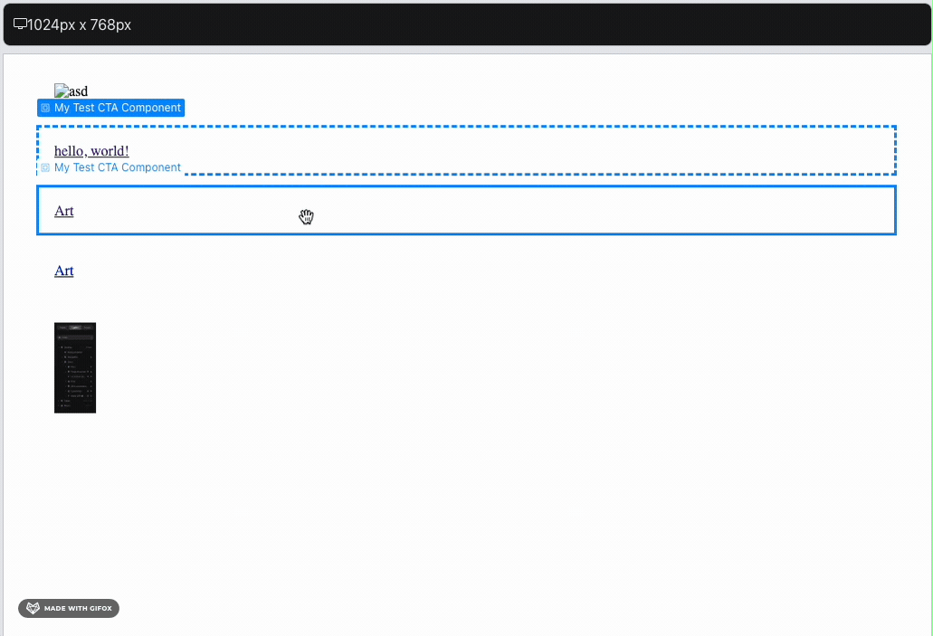
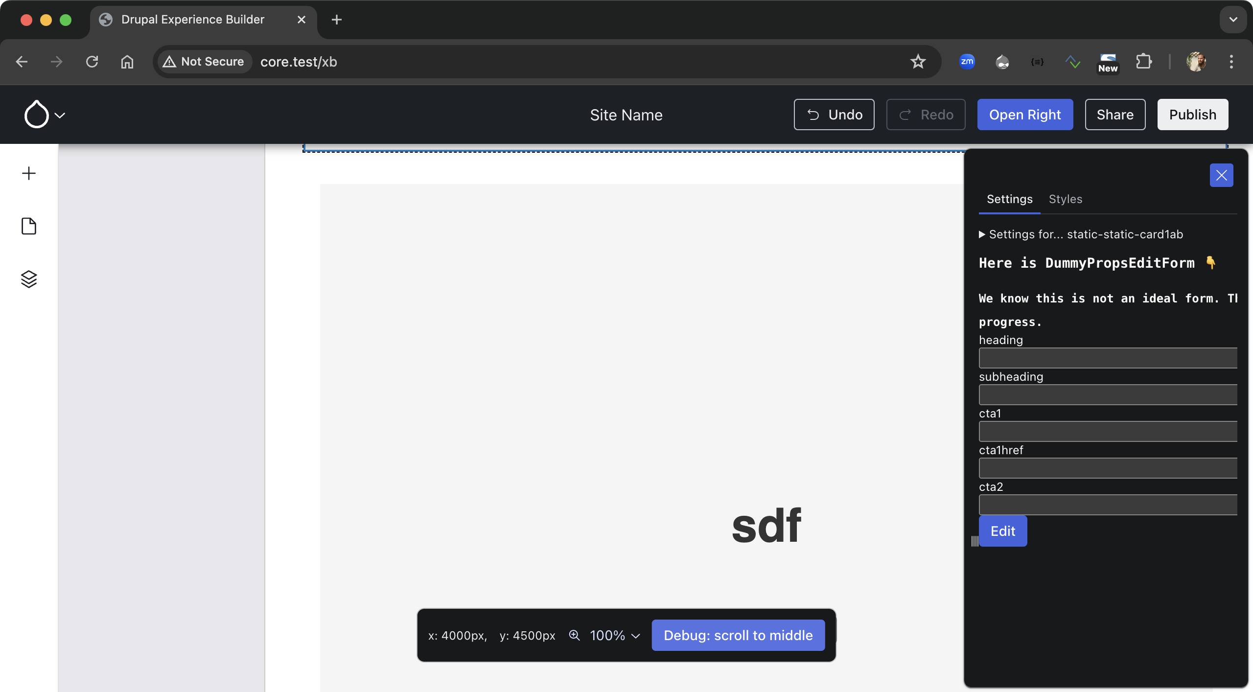
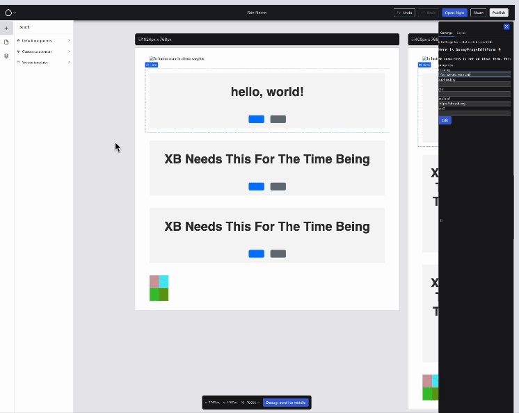
Wim Leers: XB week 11: live updates
This week started with undoing the horrors that y’all were subjected to last week: TwoTerribleTextAreasWidget featured prominently. The follow-up that I mentioned landed (Ben “bnjmnm” Mullins and I collaborated on it), which with a +110,-245 diff resulted in something that still is nowhere near a final UX, but is starting to look reasonable.
The evolved component instance props form: much simpler (it looked Frankensteinish a week ago!), by using the appropriate field widgets directly. Issue #3461422.
(Next up on that front: #3462310: Component props form: make form elements match design.)
That right sidebar is overlaid on top of the canvas, which also saw a big leap forward this week — thanks to Jesse “jessebaker” Baker, Harumi “hooroomoo” Jang, Ben “bnjmnm” Mullins and Lauri — a true team effort:
Component states in action: hover and active/focus. Issue #3460783, image by Jesse.
The images you saw last week showed actual component previews … but we cheated by using inline styles :P.
This week, Ben rectified that: CSS/JS assets are now loaded inside the preview <iframe>s.
But I saved the best for last: the last MR to land this week was Ben’s Redux integration issue … which brought with it: live updates of the component’s preview:
Live updating of component previews while the props are edited in the right sidebar! Issue #3462441, image by Ben.
This currently always requires a round trip to the server, but in many cases we’d actually be able to update the preview without a round trip (better for UX obviously!). See #3453690: [META] Real-time preview: supporting back-end infrastructure, where Lee “larowlan” Rowlands intends to work on parsing a Single-Directory Component’s Twig template into an Abstract syntax tree, which would allow eliminating that round trip in typical cases.1
I omitted less interesting MRs, but there’s one more issue that landed that deserves a mention: Ted “tedbow” Bowman and Ben landed CI: use a snapshot of core’s phpcs rules as changes in Drupal core will break MRs with limited benefit to module development, which was a very welcome addition: recently, Drupal 11 development has picked up steam … and hence several coding standards were added to Drupal core. Result: XBs phpcs CI job started failing overnight, with zero changes on our end. Doing the right thing can be painful! So, Ted and Ben changed that so we’d be notified instead: far less disruptive.
In progress/where to contribute- Experience Builder has some needs that Single-Directory Components has not had to fulfill. Lauri asked me to start developing a comprehensive plan for integrating XB with SDC: what are all the mismatches, the feature gaps, et cetera?
- Ted discovered that XB currently does not support propless SDCs — oops! This is a great first issue to contribute to XB!
- Lauri created #3463300: Implement the concept of sections within the client
- Lauri also created #3463307: Implement simplified zoom interface, which Gauravvvv quickly picked up!
- Ben created #3463610: VH units fix only works for inline styles, which seems another great first issue to contribute to XB, but this time on the front end.
- Finally, I created #3463957: “Publish” and “Share” buttons should convey they do not yet work, which was quickly picked up by fazilitehreem :)
P.S.: issues that were picked up by somebody do not exclude you from contributing too — as you can see above, almost every issue is a multi-person effort!
Missed a prior week? See all posts tagged Experience Builder.
Goal: make it possible to follow high-level progress by reading ~5 minutes/week. I hope this empowers more people to contribute when their unique skills can best be put to use!
For more detail, join the #experience-builder Slack channel. Check out the pinned items at the top!
Week 11 was July 22–28, 2024.
-
If the SDC prop value is rendered as-is, with no transformations applied, then no round trip is necessary. Otherwise, that might be needed. ↩︎
The Drop Times: Visit The DropTimes' Stall at Drupal GovCon 2024
rush @ Savannah: GNU Rush Version 2.4
Version 2.4 of GNU Rush is available for download.
New in this release:
- Use getgrouplist(3) call, if available;
- Fixes in the rush-po script;
- Bugfixes
Web Review, Week 2024-32
Let’s go for my web review for the week 2024-32.
A New Type of Neural Network Is More Interpretable - IEEE SpectrumTags: tech, ai, machine-learning, neural-networks, physics
Exciting new type of neural networks. There are limits to use them at large scale for now. Still, they have very interesting properties like the interpretability. And also, they tend to give similar performance to traditional neural networks for a smaller size.
https://spectrum.ieee.org/kan-neural-network
Tags: tech, ai, gpt
If you’re wondering what people do with chat bots, there are some clues here.
https://www.washingtonpost.com/technology/2024/08/04/chatgpt-use-real-ai-chatbot-conversations/
Tags: tech, monopoly, law
Looks like the US Department of Justice is back pushing for antitrust trials. This is likely a good thing, will it go all the way to breaking down some of the big tech companies? I doubt it but it’d probably be welcome.
https://www.theverge.com/2024/8/5/24155520/judge-rules-on-us-doj-v-google-antitrust-search-suit
Tags: tech, google, mozilla, law
Interesting guesses at what could change with the Google ruling. It doesn’t look too good for Mozilla.
https://micro.webology.dev/2024/08/06/google-search-speculation.html
Tags: tech, quic, http, networking
Clearly there’s a silent transition going on. It’s not necessarily bad that it’s on-going without making too much noise.
https://kmcd.dev/posts/yall-are-sleeping-on-http3/
Tags: tech, databases, postgresql
Definitely not as simple as it sounds. The devil is once again in the details.
https://hakibenita.com/postgresql-get-or-create
Tags: tech, debugging
You need to understand how core dumps work? This article is for you.
https://trace.yshui.dev/2024-08-copy-core-dumps.html
Tags: tech, c++, tools
Looks like an interesting tool for indexing and querying C++ code.
https://github.com/trailofbits/multiplier?tab=readme-ov-file
Tags: tech, programming, c++, safety
This is a very important distinction to keep in mind. It’s one of those source of bad mistakes in C++.
https://devblogs.microsoft.com/oldnewthing/20240802-00/?p=110091
Tags: tech, c++
Enum classes keep being improved. Nice features are already available, more might be coming through reflection in C++26.
https://www.cppstories.com/2024/enum-improvements/
Tags: tech, programming, java, safety
This would definitely be a nice change to the Java language.
https://bugs.openjdk.org/browse/JDK-8303099
Tags: tech, typescript, type-systems
The TypeScript type system is really a beast. There are little known features in this, looks definitely like one of them.
https://andreasimonecosta.dev/posts/what-the-heck-are-reverse-mapped-types/
Tags: tech, javascript, benchmarking, tools
Looks like a nice tool for benchmarking Javascript in the browser.
https://nolanlawson.com/2024/08/05/reliable-javascript-benchmarking-with-tachometer/
Tags: tech, 3d, shader
Very neat technique for global illumination. Very effective but still has some issues.
https://mini.gmshaders.com/p/radiance-cascades
Tags: tech, tools, git, version-control, codereview
I like the idea of getting all the review comments back into Git once things are merged. This works offline, makes you less dependent on the forge for historical data etc. Now we’d probably need to have the notes feature easier to use somehow.
https://wouterj.nl/2024/08/git-notes
Tags: tech, tools, git, version-control, quality
Maybe we could store metrics about the code in the history as well? This would indeed reduce vendor lock-in. This tool makes it easy. Unsurprisingly seems built upon git notes.
https://dev.to/jdrouet/build-metrics-and-budgets-with-git-metrics-4pb4
Tags: tech, engineering, productivity, metrics
Aren’t we loosing something if we focus on productivity numbers too much? A good reminder that intrinsic motivation is an important driver in people behavior. I wouldn’t throw all the metrics out of the door but they’d better be a limited amount and they’d better be informative rather than objectives.
https://tidyfirst.substack.com/p/humans-data
Bye for now!
Real Python: The Real Python Podcast – Episode #216: Learning Through Building the Black Python Devs Community
What hurdles must be cleared when starting an international organization? How do you empower others in a community by sharing responsibilities? This week on the show, we speak with Jay Miller about Black Python Devs.
[ Improve Your Python With 🐍 Python Tricks 💌 – Get a short & sweet Python Trick delivered to your inbox every couple of days. >> Click here to learn more and see examples ]
The Drop Times: Elevating Drupal Beyond a CMS: Dominique De Cooman
mark.ie: My Drupal Core Contributions for week-ending August 9th, 2024
Here's what I've been working on for my Drupal contributions this week. Thanks to Code Enigma for sponsoring the time to work on these.
PyPy: Conda-forge proposes sunsetting support for PyPy
Conda-forge has kindly been providing support for PyPy since 2019. The conda-forge team has been very patient and generous with resources, but it seems the uptake of PyPy has not justified the effort. Major packages still are not available on PyPy, others find it hard to update versions. We don't get much feedback at all about people using PyPy, and even less about PyPy on conda-forge. The conda-forge team has proposed sunsetting PyPy going forward, which means current packages would remain but no new packages would be built. If you have an opinion, you can comment on that PR, or on this blog post.
Since conda-forge supports PyPy3.9 but not PyPy3.10, we have continued releasing PyPy3.9 even though we typically support only one version of PyPy3. With the sunsetting proposal, we will not release any more updates to PyPy3.9. I opened a poll about the intention to drop PyPy3.9. If you have an opinion, please chime in.
Matt Layman: Go Standard Library App - Building SaaS #197.4
Pages
Recent Publications
- Managing Hidden Dependencies in OO Software: a Study Based on Open Source Projects
- Open Source Communities as Liminal Ecosystems
- Investigating developers' email discussions during decision-making in Python language evolution
- Developers, Quality Control and Download Volume in Open Source Software (OSS) Projects
FLOSS Project Planets
- Bounteous.com: Upgrading to Drupal 10 (And Beyond) With Composer
- FSF Blogs: Free software is vital for the public and state-run infrastructure of a free society
- Free software is vital for the public and state-run infrastructure of a free society
- Kdenlive Café in December
- PyPodcats: Episode 7: With Anna Makarudze
FLOSS Research
- Celebrating 5 years at the Open Source Initiative: a journey of growth, challenges, and community engagement
- Highlights from the Digital Public Goods Alliance Annual Members Meeting 2024
- Give Your Input on the State of Open Source Survey
- Open Data and Open Source AI: Charting a course to get more of both
- The Open Source Initiative and the Eclipse Foundation to Collaborate on Shaping Open Source AI (OSAI) Public Policy