
FLOSS Project Planets
LN Webworks: Integrating Drupal And Tailwind CSS: Step-By-Step Guide
It’s hectic and time-consuming when it comes to making something that takes a long time. Yes, we are talking about CSS stylesheets. It’s not easy to design a website because it’s not ‘effortless’.
In this blog, we will talk about the Integration of Drupal and Tailwood CSS to make this process a little bit easier for you.
A brief About Tailwind CSSTailwind CSS adopts a utility-first approach rather than building a class for the component. Tailwind CSS is a utility-first approach that makes creating applications faster and easier
Tailwind CSS offers limited benefits but assures you the flexibility and power to create your unique site.
Specbee: How to set up Apache Solr Plugin on Ubuntu in a Lando environment and configure Search API Solr in Drupal
Talking Drupal: Talking Drupal #463 - Drupal vs DIY Site Builders
Today we are talking about DIY Site Builders, what are the benefits over Drupal (If Any), and When using Drupal makes sense with guest Ivan Stegic. We’ll also cover Drupal 11 as our module of the week.
For show notes visit: www.talkingDrupal.com/463
Topics- What is a DIY site builder
- Does TEN7 use DIY site builders
- How are DIY site builders better than Drupal
- Are they less expensive than Drupal
- HAve you ever suggested a site builder to a client
- What does a migration from a site builder look like
- Do you think starshot will make Drupal competitive with site builders
- Workspaces Extra
- Talking Drupal 451 - Just say Drupal
- Shopify
- Webflow
- Wix
- Squarespace
- Wordpress vip
- Cosmic.build
- Preshow:
Ivan Stegic - ten7.com ivanstegic
HostsNic Laflin - nLighteneddevelopment.com nicxvan John Picozzi - epam.com johnpicozzi Josh Miller - joshmiller
MOTW CorrespondentMartin Anderson-Clutz - mandclu.com mandclu
- Brief description:
- Have you been wanting a version of Drupal that can use Workspaces, Recipes, and Single Directory Components, while running all the latest versions of its underlying technologies? Drupal 11 is all of that and more
- Module name/project name:
- Brief history
- How old: created on Aug 2 by catch of Tag1 and Third & Grove
- Module features and usage
- Limited additions vs 10.3: by design to make the transition easier
- Mostly in the recipes API, e.g. new config actions
- Recap of new features vs. 10.0
- Workspaces
- Revisions and workflow are possible in the UI for Blocks and Taxonomy Terms
- UI updates for creating and reusing fields, as well as bulk content operations
- New Access Policy API and Single Directory Components
- New Navigation and Announcements Feed modules
- Contrib support out of the gate: about ⅔ of the top 200 modules already support Drupal 11
- Adding modules that Rector estimates will only need info.yml or automated fixes brings us to over 80% of the top 200, or about 75% of all Drupal 10-compatible projects on Drupal.org
- Updated dependencies: PHP 8.3, Symfony 7, CKEditor 5 42.0,2, Twig 3.9, Yarn 4, jQuery 4.0.0-beta, jQuery UI 1.14-beta.2 and more
- Modules moved to contrib (smaller core):
- Actions UI
- Activity Tracker
- Book
- Forum
- Statistics
- Tour
- Drupal 10 will receive maintenance support until mid-2026, so the community created this release of Drupal 11 early to give sites as much time as possible to make the transition, in this case almost 2 years!
- Limited additions vs 10.3: by design to make the transition easier
Scarlett Gately Moore: KDE, Kubuntu, Debian Qt6 updates plus Kubuntu Noble .1 updates.
Another loss last week of a friend. I am staying strong and working through it. A big thank you to all of you that have donated to my car fund, I still have a long way to go. I am not above getting a cheap old car, but we live in sand dunes so it must be a cheap old car with 4×4 to get to my property. A vehicle is necessary as we are 50 miles away from staples such as food and water. We also have 2 funerals to attend. Please consider a donation if my work is useful to you. https://gofund.me/1e784e74 All of my work is currently unpaid work, as I am between contracts. Thank you for your consideration. Now onto the good stuff, last weeks work. It was another very busy week with Qt6 packaging in Debian/Kubuntu and KDE snaps. I also have many SRUs for Kubuntu Noble .1 release that needs their verification done.
Kubuntu:
- See Debian for the qt6 Plasma / applications work.
- Many SRUs in verification stage, please help test these: https://wiki.ubuntu.com/StableReleaseUpdates#Verification
- https://bugs.launchpad.net/ubuntu/+source/tellico/+bug/2065915 – needs testing on ARM and there are many packages in that bug.
- https://bugs.launchpad.net/ubuntu/+source/kubuntu-meta/+bug/2065465 Fix systray icons for third party apps like spotify
- https://bugs.launchpad.net/ubuntu/+source/plasma-workspace/+bug/1629543 Lightdm login manager crash when plasma selected.
- https://bugs.launchpad.net/ubuntu/+source/ark/+bug/2068491 Opening 7zip files in ark.
- https://bugs.launchpad.net/ubuntu/+source/merkuro/+bug/2063936 Merkuro fails to start. Verification done, but more testers welcome.
- https://bugs.launchpad.net/bugs/2066275 SDDM fails to boot after second boot. This SRU has been released!
- https://bugs.launchpad.net/ubuntu/+source/neochat/+bug/2061116 Neochat fails to start.
Debian:
Starting the salvage process for kdsoap which is blocking a long line of packages, notably kio-extras.
- qtmpv – in NEW
- arianna – in NEW
- xwaylandvideobridge – NEW
- futuresql – NEW
- kpat WIP – failing tests
- kdegraphics-thumbnailers (WIP)
- khelpcenter – experimental
- kde-inotify-survey – experimental
- ffmpegthumbs – experimental
- kdialog – experimental
- kwalletmanager – experimental
- libkdegames – pushed some fixes – experimental
- Tokodon – Done, but needs qtmpv to pass NEW
- Gwenview – WIP needs – kio-extras (blocked)
KDE Snaps:
Please note: Please help test the –edge snaps so I can promote them to stable.
- Arianna stable https://snapcraft.io/arianna
- Kfind stable https://snapcraft.io/kfind
- Kclock –edge https://snapcraft.io/kclock
- Kigo –edge https://snapcraft.io/kigo
- Kimagemapeditor –edge https://snapcraft.io/kimagemapeditor
- Kspacedual –edge https://snapcraft.io/kspaceduel
- Picmi –edge https://snapcraft.io/picmi
- lskat –edge https://snapcraft.io/lskat
- Ksudoku –edge https://snapcraft.io/ksudoku
- Ksquares –edge https://snapcraft.io/ksquares
- Juk –edge https://snapcraft.io/juk
- Kalgebra –edge https://snapcraft.io/kalgebra
- Ktuberling –edge https://snapcraft.io/ktuberling
- Ruqola –edge https://snapcraft.io/ruqola
WIP Snaps or MR’s made
- Kirigami-gallery ( building )
- Kiriki (building)
- Kiten (building)
- kjournald (Building)
- Kdevelop (WIP)
- Kdenlive (building)
- KHangman (WIP)
- Kubrick (WIP)
- Palapeli (Manual review in store dbus)
- Kanagram (WIP)
- Labplot (WIP)
- Kjumpingcube (MR)
- Klettres (MR)
- Kajongg –edge (Broken, problem with pyqt)
- Dragon –edge ( Broken, dbus fails)
- Ghostwriter –edge ( Broken, need to workout Qt webengine obscure way of handling hunspell dictionaries.)
- Kasts –edge ( Broken, portal failure, testing some plugs)
- Kbackup –edge ( Needs auto-connect udisks2, added home plug)
- Kdebugsettings –edge ( Added missing personal-files plug, will need approval)
- KDiamond –edge ( sound issues )
- Angelfish –edge https://snapcraft.io/angelfish ( Crashes on first run, but runs fine after that.. looking into it)
- Qrca –edge ( needs snap connect qrca:camera camera until auto-connect approved, will remain in –edge until official release)
KDE, Kubuntu, Debian Qt6 updates plus Kubuntu Noble .1 updates.
Another loss last week of a friend. I am staying strong and working through it. A big thank you to all of you that have donated to my car fund, I still have a long way to go. I am not above getting a cheap old car, but we live in sand dunes so it must be a cheap old car with 4×4 to get to my property. A vehicle is necessary as we are 50 miles away from staples such as food and water. We also have 2 funerals to attend. Please consider a donation if my work is useful to you. https://gofund.me/1e784e74 All of my work is currently unpaid work, as I am between contracts. Thank you for your consideration. Now onto the good stuff, last weeks work. It was another very busy week with Qt6 packaging in Debian/Kubuntu and KDE snaps. I also have many SRUs for Kubuntu Noble .1 release that needs their verification done.
Kubuntu:
- See Debian for the qt6 Plasma / applications work.
- Many SRUs in verification stage, please help test these: https://wiki.ubuntu.com/StableReleaseUpdates#Verification
- https://bugs.launchpad.net/ubuntu/+source/tellico/+bug/2065915 – needs testing on ARM and there are many packages in that bug.
- https://bugs.launchpad.net/ubuntu/+source/kubuntu-meta/+bug/2065465 Fix systray icons for third party apps like spotify
- https://bugs.launchpad.net/ubuntu/+source/plasma-workspace/+bug/1629543 Lightdm login manager crash when plasma selected.
- https://bugs.launchpad.net/ubuntu/+source/ark/+bug/2068491 Opening 7zip files in ark.
- https://bugs.launchpad.net/ubuntu/+source/merkuro/+bug/2063936 Merkuro fails to start. Verification done, but more testers welcome.
- https://bugs.launchpad.net/bugs/2066275 SDDM fails to boot after second boot. This SRU has been released!
- https://bugs.launchpad.net/ubuntu/+source/neochat/+bug/2061116 Neochat fails to start.
Debian:
Starting the salvage process for kdsoap which is blocking a long line of packages, notably kio-extras.
- qtmpv – in NEW
- arianna – in NEW
- xwaylandvideobridge – NEW
- futuresql – NEW
- kpat WIP – failing tests
- kdegraphics-thumbnailers (WIP)
- khelpcenter – experimental
- kde-inotify-survey – experimental
- ffmpegthumbs – experimental
- kdialog – experimental
- kwalletmanager – experimental
- libkdegames – pushed some fixes – experimental
- Tokodon – Done, but needs qtmpv to pass NEW
- Gwenview – WIP needs – kio-extras (blocked)
KDE Snaps:
Please note: Please help test the –edge snaps so I can promote them to stable.
- Arianna stable https://snapcraft.io/arianna
- Kfind stable https://snapcraft.io/kfind
- Kclock –edge https://snapcraft.io/kclock
- Kigo –edge https://snapcraft.io/kigo
- Kimagemapeditor –edge https://snapcraft.io/kimagemapeditor
- Kspacedual –edge https://snapcraft.io/kspaceduel
- Picmi –edge https://snapcraft.io/picmi
- lskat –edge https://snapcraft.io/lskat
- Ksudoku –edge https://snapcraft.io/ksudoku
- Ksquares –edge https://snapcraft.io/ksquares
- Juk –edge https://snapcraft.io/juk
- Kalgebra –edge https://snapcraft.io/kalgebra
- Ktuberling –edge https://snapcraft.io/ktuberling
- Ruqola –edge https://snapcraft.io/ruqola
WIP Snaps or MR’s made
- Kirigami-gallery ( building )
- Kiriki (building)
- Kiten (building)
- kjournald (Building)
- Kdevelop (WIP)
- Kdenlive (building)
- KHangman (WIP)
- Kubrick (WIP)
- Palapeli (Manual review in store dbus)
- Kanagram (WIP)
- Labplot (WIP)
- Kjumpingcube (MR)
- Klettres (MR)
- Kajongg –edge (Broken, problem with pyqt)
- Dragon –edge ( Broken, dbus fails)
- Ghostwriter –edge ( Broken, need to workout Qt webengine obscure way of handling hunspell dictionaries.)
- Kasts –edge ( Broken, portal failure, testing some plugs)
- Kbackup –edge ( Needs auto-connect udisks2, added home plug)
- Kdebugsettings –edge ( Added missing personal-files plug, will need approval)
- KDiamond –edge ( sound issues )
- Angelfish –edge https://snapcraft.io/angelfish ( Crashes on first run, but runs fine after that.. looking into it)
- Qrca –edge ( needs snap connect qrca:camera camera until auto-connect approved, will remain in –edge until official release)
FSF Events: Free Software Directory meeting on IRC: Friday, August 16, starting at 12:00 EDT (16:00 UTC)
PyCharm: PyCharm 2024.2 Is Here: Improvements for Jupyter Notebooks, Databricks Integration, New AI Assistant Features, and More!
Offering a wide range of new and improved functionality, including Hugging Face integration, new AI Assistant features, a new default UI, and an overall better user experience, PyCharm 2024.2 is a must for anyone looking to increase their productivity.
Learn about all the updates on our What’s New page, download the latest version from our website, or update your current version through our free Toolbox App.
Download PyCharm 2024.2 PyCharm 2024.2 key features Databricks integration PROPyCharm now provides direct integration with Databricks via a plugin. You can connect to a Databricks cluster, execute scripts and notebooks as workflows, execute files directly in a Spark shell on a cluster, and monitor the progress – all from the comfort of your IDE.
This integration allows you to harness the power of your IDE when working with Databricks, making the process faster and easier.
Hugging Face integration PROPyCharm 2024.2 can now suggest the most relevant Hugging Face models based on your use case. When you select a model, the IDE will suggest inserting a code snippet that allows you to use it directly in the open file, and PyCharm will download and install any missing dependencies automatically.
You can also identify unused models installed on your machine and delete them to free up disk space directly from the IDE.
Additionally, you can inspect your Hugging Face Datasets library data as an interactive dataframe, utilizing features like the chart view, pagination, and the ability to sort and export tables.
Read more Jupyter notebooks PROInstantly preview the value of a chosen variable simply by hovering over the variable’s line. You no longer need to use the debugger or print statements!
Furthermore, you can now expand and collapse cells, as well as run them straight from the gutter. Additionally, cells now display their statuses and assigned tags.
All these improvements are designed to make working with Jupyter notebooks in PyCharm seamless, fast, and efficient.
AI cells in Jupyter notebooksWith our new AI cell option, you can add prompts directly inside your notebooks and work with AI Assistant right from there. A light bulb icon next to the AI cell provides suggestions about the next steps in your data analysis workflow.
One-click dataframe visualizationVisualize your dataframes with the help of AI Assistant, which now provides suggestions about the graphs and plots most suitable to your context.
AI AssistantJetBrains AI Assistant 2024.2 enhances cloud-based code completion with faster, more accurate suggestions and a better UX, including syntax highlighting and the option to accept suggestions incrementally. The AI chat now uses the latest GPT-4o model and supports chat references and semantic search.
New features include AI integration in the Terminal tool window for command generation, AI-assisted VCS conflict resolution, and customizable prompts for documentation and unit test creation.
Learn about these and other AI Assistant enhancements in this dedicated blog post.
Database tools PRO New AI Assistant featuresWith the text-to-SQL feature, you can generate SQL code directly in the editor by clicking Generate Code with AI and entering your prompt. You can accept, regenerate, or refine the code, and take it to the AI chat if you have further questions.
Additionally, AI Assistant can help with modifying tables, allowing you to request changes like switching all VARCHAR data types to CHAR.
It can also help you understand and fix SQL problems, suggesting explanations and fixes.
Read more User experience Preview option in Search EverywhereThe Search Everywhere dialog now includes an option to preview the codebase elements you’re searching for, offering additional context and making it easier to navigate through your project.
Improved full line code completion PROIn 2024.2, full line code completion suggestions now include code highlighting, and new shortcuts allow you to accept individual words or entire lines from longer suggestions. We’ve also refined how accepted changes are integrated into your code, eliminating any formatting issues.
Run/Debug String variable visualizers for JSON, XML, and other formatsDebugging and browsing long string variables with complex data formats is now much easier. The updated debugger offers properly formatted visualizations for string variables with strings encoded in JSON, XML, HTML, JWT, and URL.
Frameworks and technologies PRO GraalJS as the execution engine for the HTTP ClientWe’ve upgraded the JavaScript execution engine used in the HTTP Client to GraalJS. This allows you to use all GraalJS features, including full support for the ECMAScript 2023 specification, when testing endpoints with PyCharm’s HTTP Client and using JavaScript in .http files to handle the results.
HTTP Client improvementsIn the HTTP Client, we’ve added XPath functionality for querying and manipulating XML and HTML documents, support for iterating through collections using JSONPath to automate requests, and the ability to create and add custom API methods effortlessly.
Enhanced Terraform supportWe’ve enhanced PyCharm’s Terraform support with full line code completion, improved context-aware code completion, refined syntax highlighting, and better error detection with quick-fix suggestions. Additionally, a quick documentation feature now provides instant tooltips, offering immediate information to streamline your Terraform workflow.
Frontend PRO Improved support for major web frameworksPyCharm can now resolve paths for frameworks that use file-system-based routing. It can also resolve link paths based on your project’s file system, providing autocompletion and navigation for Next.js, Nuxt, SvelteKit, and Astro. There is also support for new Svelte 5 snippets and render tags.
Additionally, we’ve implemented language server protocol (LSP) support for Astro and upgraded the Vue LSP to Vue Language Service v2, improving code completion and the overall developer experience.
Ability to run and debug TypeScript files directlyYou can now run and debug TypeScript files from different entry points, including the file context menu, the Run widget, and the Current File configuration.
Remote development PRO Reverse port forwardingWith reverse port forwarding, you can now connect a remote IDE to ports available on the client machine. This is particularly useful for mobile development and connecting to local databases.
Download PyCharm 2024.2These are all the key features of this release, but there’s much more to explore! Visit our What’s New page or release notes for the full breakdown and additional details about the features mentioned here.
If you encounter any problems, please report them in our issue tracker so we can address them promptly.
Connect with us on X (formerly Twitter) to share your thoughts on PyCharm 2024.2. We’re looking forward to hearing them!
Real Python: Python News Roundup: August 2024
In July, there was some exciting news for the Python community as the Python core development team released versions 3.13.0b4 and 3.13.0rc1 of the language. The 3.13.0b4 release marked the end of the beta phase and paved the way for the release candidate phase.
Note that 3.13.0rc1 is a pre-release, so you shouldn’t use it for production environments. However, it provides a great way to try some new and exciting language features.
There’s also great some news from the Python Software Foundation, PyOhio 2024, and the Python ecosystem.
Let’s dive into the most exciting Python news from last month!
Python 3.13.0b4 and 3.13.0rc1Python 3.13 has reached its fourth beta release, marking the end of the beta phase. Beta releases serve to test new features and bug fixes. However, it’s important to note that this is a preview release and it isn’t recommended for use in production environments.
If you’re a library maintainer, you’re encouraged to test your code with this new version so you can prepare it to support the latest features of the language.
Note: To learn more about pre-releases, check out the How Can You Install a Pre-Release Version of Python? tutorial.
One of the most significant new features of Python 3.13 is the improved interactive interpreter or REPL, which now provides several cool features, including:
- Colorized prompts
- Multiline editing with history preservation
- Interactive help browsing with F1 and a separate command history
- History browsing with F2
- Paste mode for larger blocks of code with F3
- REPL-specific commands like help, exit, and quit without the call parentheses
This is exciting news! The standard REPL up until Python 3.13 was lacking, and sometimes it was necessary to install a third-party tool like bpython or IPython to compensate.
Again, with this release, the beta phase has officially ended, and the first release candidate—3.13.0rc1—is considered the penultimate release preview. In this release candidate phase, only bug fixes are allowed.
The second candidate, which is the last planned release preview, should be out on September 3, 2024, and the official release of 3.13 should be ready on October 1, 2024. Only more excitement lies ahead!
The Python Software Foundation (PSF) Shares Great News Read the full article at https://realpython.com/python-news-august-2024/ »[ Improve Your Python With 🐍 Python Tricks 💌 – Get a short & sweet Python Trick delivered to your inbox every couple of days. >> Click here to learn more and see examples ]
Week 11 recap - Final Stretch
The Drop Times: Drupal GovCon 2024: The Heartbeat of the DC Drupal community
Mike Driscoll: Creating Progress Bars in Your Terminal with Python and Textual
The Textual package is a great way to create GUI-like applications with Python in your terminal. These are known as text-based user interfaces or TUIs. Textual has many different widgets built-in to the framework.
One of those widgets is the ProgressBar. If you need to show the progress of a download or long-running process, then you will probably want to use a progress bar or some kind of spinner widget to show the user that your application is working.
This tutorial will show you how to create a simple progress bar with Textual!
InstallationIf you do not have Textual installed yet, you can get it by using Python’s handy pip tool. Open up your terminal and run the following command there:
python -m pip install textualTextual will get installed, along with all its dependencies. You may want to create a virtual environment first and install Textual there.
Creating a ProgressBar in TextualCreating a progress bar with Textual is pretty straightforward. The following code is based on an example from the Textual documentation. The main difference is that this version uses a button to start the timer, simulating a download or some other long-running process rather than catching a key event.
You can copy this code into your favorite Python editor and give it a quick study:
# progressbar_demo.py from textual.app import App, ComposeResult from textual.containers import Center, Middle from textual.timer import Timer from textual.widgets import Button, ProgressBar class Progress(App[None]): timer = Timer def compose(self) -> ComposeResult: with Center(): with Middle(): yield ProgressBar() yield Button("Start") def on_mount(self) -> None: """ Set up the timer to simulate progress """ self.timer = self.set_interval(1 / 10, self.advance_progressbar, pause=True) def advance_progressbar(self) -> None: """ Called to advance the progress bar """ self.query_one(ProgressBar).advance(1) def on_button_pressed(self) -> None: """ Event handler that is called when button is pressed """ self.query_one(ProgressBar).update(total=100) self.timer.resume() if __name__ == "__main__": app = Progress() app.run()The compose() method is kind of fun as it uses both the Center() and the Middle() containers to position the widgets in the middle of the terminal. You then set up the timer object in on_mount() and you start the timer in on_button_pressed()which is the Button widget’s event handler.
When you run this code, you will initially see what’s known as an indeterminate progress bar. What that means is that Textual doesn’t have any information about how long the progress is, so the progress bar just shows a kind of “bouncing” or “cycling” progress:
When you press the “Start” button, you will see the progress bar go from 0-100%, and the text fields to the right will update as well:
If you want to make your progress bar stand out, add a gradient. A gradient will make the colors of the progress bar change over time and make the widget look neat!
Wrapping UpAdding a progress bar or simply showing some kind of informational widget that lets the user know your application is working is always a good idea. You don’t want the user to think the application has crashed or frozen. The user might be forced to close the application and lose their information after all!
Fortunately, Textual makes adding a progress bar easy. Not only is it easy, but the progress bar is easy to update so you can accurately give the user a sense of when the work will be done. Give it a try and see what you think!
Related ReadingWant to learn more about Textual? Check out the following articles:
The post Creating Progress Bars in Your Terminal with Python and Textual appeared first on Mouse Vs Python.
The Drop Times: Latest Breakthroughs in the Drupal Starshot Initiative
Zato Blog: How to correctly integrate APIs in Python
Understanding how to effectively integrate various systems and APIs is crucial. Yet, without a dedicated integration platform, the result will be brittle point-to-point, spaghetti integrations, that never lead to good outcomes.
➤ Read this article about Zato, an open-source integration platform in Python, for an overview of what to avoid and how to do it correctly instead.
More blog posts➤Golems GABB: Scaling and Performance Optimization of Drupal
The future is not distant anymore, so what kind of "good Drupal performance and scalability" can we expect in 2024? Moreover, what implementations can be done via Drupal's features and options to impress an online audience?
Nowadays, in the era of digital content, a website should be ultramodern in both presentation and performance. Consumers prefer easy experiences. Hence, the ability of an organization to do this for them is a critical factor in service delivery. Regarding the user side of the services, sites should hold up with rapid traffic growth, constantly upgrade, and provide users with a wide range of features.
Moreover, such a growing level of cross-communication may not only meet those expectations but also go far beyond them to help organizations grow in the digital domain.
Freexian Collaborators: Monthly report about Debian Long Term Support, July 2024 (by Roberto C. Sánchez)
Like each month, have a look at the work funded by Freexian’s Debian LTS offering.
Debian LTS contributorsIn July, 13 contributors have been paid to work on Debian LTS, their reports are available:
- Bastien Roucariès did 20.0h (out of 20.0h assigned).
- Chris Lamb did 18.0h (out of 18.0h assigned).
- Daniel Leidert did 5.0h (out of 4.0h assigned and 6.0h from previous period), thus carrying over 5.0h to the next month.
- Guilhem Moulin did 8.75h (out of 4.5h assigned and 15.5h from previous period), thus carrying over 11.25h to the next month.
- Lee Garrett did 51.5h (out of 10.5h assigned and 43.0h from previous period), thus carrying over 2.0h to the next month.
- Lucas Kanashiro did 5.0h (out of 5.0h assigned and 15.0h from previous period), thus carrying over 15.0h to the next month.
- Markus Koschany did 40.0h (out of 40.0h assigned).
- Ola Lundqvist did 4.0h (out of 10.0h assigned and 14.0h from previous period), thus carrying over 20.0h to the next month.
- Roberto C. Sánchez did 5.0h (out of 5.25h assigned and 6.75h from previous period), thus carrying over 7.0h to the next month.
- Santiago Ruano Rincón did 6.0h (out of 16.0h assigned), thus carrying over 10.0h to the next month.
- Sean Whitton did 2.25h (out of 6.0h assigned), thus carrying over 3.75h to the next month.
- Sylvain Beucler did 39.5h (out of 2.5h assigned and 51.0h from previous period), thus carrying over 14.0h to the next month.
- Thorsten Alteholz did 11.0h (out of 11.0h assigned).
In July, we have released 1 DLA.
August will be the month that Debian 11 makes the transition to LTS. Our contributors have already been hard at work with preparatorty tasks and also with making contributions to packages in Debian 11 in close collaboration with the Debian security team and package maintainers. As a result, users and sponsors should not observe any especially notable differences as the transition occurs.
While only one DLA was released in July (as a result of the transitional state of Debian 11 “bullseye”), there were some notable highlights. LTS contributor Guilhem Moulin prepared an update of libvirt for Debian 11 (in collaboration with the Old-Stable Release Managers and the Debian Security Team) to fix a number of outstanding CVEs which did not rise to the level of a DSA by the Debian Security Team. The update prepared by Guilhem will be included in Debian 11 as part of the final point release at the end of August, one of the final transition steps by the Release Managers as Debian 11 moves entirely to the LTS Team’s responsibility. Notable work was also undertaken by contributors Lee Garrett (fixes on the ansible test suite and a bullseye update), Lucas Kanashiro (Rust toolchain, utilized by the clamav, firefox-esr, and thunderbird packages), and Sylvain Beucler (fixes on the ruby2.5/2.7 test suites and CI infrastructure), which will help improve the quality of updates produced during the next LTS cycle.
June was the final month of LTS for Debian 10 (as announced on the debian-lts-announce mailing list). No additional Debian 10 security updates will be made available on security.debian.org.
However, Freexian and its team of paid Debian contributors will continue to maintain Debian 10 going forward for customers of the Extended LTS offer. Subscribe right away if you sill have Debian 10 systems which must be kept secure (and which cannot yet be upgraded).
Thanks to our sponsorsSponsors that joined recently are in bold.
- Platinum sponsors:
- TOSHIBA (for 106 months)
- Civil Infrastructure Platform (CIP) (for 74 months)
- VyOS Inc (for 38 months)
- Gold sponsors:
- Roche Diagnostics International AG (for 116 months)
- Linode (for 110 months)
- Babiel GmbH (for 100 months)
- Plat’Home (for 99 months)
- CINECA (for 74 months)
- University of Oxford (for 56 months)
- Deveryware (for 43 months)
- EDF SA (for 28 months)
- Dataport AöR (for 3 months)
- Silver sponsors:
- Domeneshop AS (for 121 months)
- Nantes Métropole (for 115 months)
- Univention GmbH (for 107 months)
- Université Jean Monnet de St Etienne (for 107 months)
- Ribbon Communications, Inc. (for 101 months)
- Exonet B.V. (for 91 months)
- Leibniz Rechenzentrum (for 85 months)
- Ministère de l’Europe et des Affaires Étrangères (for 69 months)
- Cloudways by DigitalOcean (for 58 months)
- Dinahosting SL (for 56 months)
- Bauer Xcel Media Deutschland KG (for 50 months)
- Platform.sh SAS (for 50 months)
- Moxa Inc. (for 44 months)
- sipgate GmbH (for 42 months)
- OVH US LLC (for 40 months)
- Tilburg University (for 40 months)
- GSI Helmholtzzentrum für Schwerionenforschung GmbH (for 31 months)
- Soliton Systems K.K. (for 28 months)
- THINline s.r.o. (for 4 months)
- Bronze sponsors:
- Evolix (for 121 months)
- Seznam.cz, a.s. (for 121 months)
- Intevation GmbH (for 118 months)
- Linuxhotel GmbH (for 118 months)
- Daevel SARL (for 117 months)
- Bitfolk LTD (for 116 months)
- Megaspace Internet Services GmbH (for 116 months)
- Greenbone AG (for 115 months)
- NUMLOG (for 115 months)
- WinGo AG (for 114 months)
- Entr’ouvert (for 105 months)
- Adfinis AG (for 103 months)
- Tesorion (for 98 months)
- GNI MEDIA (for 97 months)
- Laboratoire LEGI - UMR 5519 / CNRS (for 97 months)
- Bearstech (for 89 months)
- LiHAS (for 89 months)
- Catalyst IT Ltd (for 84 months)
- Supagro (for 79 months)
- Demarcq SAS (for 78 months)
- Université Grenoble Alpes (for 64 months)
- TouchWeb SAS (for 56 months)
- SPiN AG (for 53 months)
- CoreFiling (for 49 months)
- Institut des sciences cognitives Marc Jeannerod (for 44 months)
- Observatoire des Sciences de l’Univers de Grenoble (for 40 months)
- Tem Innovations GmbH (for 35 months)
- WordFinder.pro (for 34 months)
- CNRS DT INSU Résif (for 33 months)
- Alter Way (for 26 months)
- Institut Camille Jordan (for 16 months)
- SOBIS Software GmbH
Freexian Collaborators: Debian Contributions: autopkgtest/incus builds, live-patching, Salsa CI, Python 3.13 (by Stefano Rivera)
Contributing to Debian is part of Freexian’s mission. This article covers the latest achievements of Freexian and their collaborators. All of this is made possible by organizations subscribing to our Long Term Support contracts and consulting services.
autopkgtest/Incus build streamlining, by Colin WatsonColin contributed a change to allow maintaining Incus container and VM images in parallel. Both of these are useful (containers are faster, but some tests need full machine isolation), and the build tools previously didn’t handle that very well.
This isn’t yet in unstable, but once it is, keeping both flavours of unstable images up to date will be a simple matter of running this regularly:
RELEASE=sid autopkgtest-build-incus images:debian/trixie RELEASE=sid autopkgtest-build-incus --vm images:debian/trixie Linux live-patching, by Santiago Ruano RincónIn collaboration with Emmanuel Arias, Santiago continued the work on the support for applying security fixes to the Linux kernel in Debian, without the need to reboot the machine. As mentioned in the previous month report, kpatch 0.9.9-1 (and 0.9.9-2 afterwards) was uploaded to unstable in July, closing the Intent to Salvage (ITS) bug. With this upload, the remaining RC bugs were solved, and kpatch was able to transition to Debian testing recently. Kpatch is expected to be an important component in the live-patching support, since it makes it easy to build a patch as a kernel module. Emmanuel and Santiago continued to work on the design for Linux live-patching and presented the current status in the DebConf24 presentation.
Salsa CI, by Santiago Ruano RincónTo be able to add RISC-V support and to avoid using tools not packaged in Debian (See #331), the Salsa CI pipeline first needed to move away from kaniko to build the images used by the pipeline. Santiago created a merge request to use buildah instead, and it was merged last month. Santiago also prepared a couple of more MRs related to how the images are built: initial RISC-V support, that should be merged after improving how built images are tested. The switch to buildah introduced a regression in the work-in-progress MR that adds new build image so the build job can run sbuild. Santiago hopes to address this regression and continue with the sbuild-related MRs in August.
Additionally, Santiago also contributed to the install docker-cli instead of docker.io in the piuparts image MR, and reviewed others such as reprotest: Add –append-build-command option, fix failure at manual pipeline run when leaving RELEASE variable empty and Fix image not found error on image building stage.
Python 3.13 Betas, by Stefano RiveraAs Python 3.13 is approaching the first release, Stefano has been uploading the beta releases to Debian unstable. Most of these have uncovered small bugs that needed to be investigated and fixed.
Stefano also took the time to review the current patch set against cPython in Debian.
Python 3.13 isn’t marked as a supported Python release in Debian’s Python tooling, yet, so nothing has been built against it, yet. Now that the Python 3.12 transition has completed, the next task will be to start trying to build Debian’s Python module packages against Python 3.13, to estimate the work required to transition to 3.13 in unstable.
Miscellaneous contributions- Carles Pina updated the packages python-asyncclick, python-pyaarlo and prepared updates for python-ring-doorbell and simplemonitor.
- Carles Pina updated (reviewing or translating) Catalan translations for adduser, apt-listchanges, debconf and shadow.
- Colin merged OpenSSH 9.8, and prepared a corresponding release note for DSA support now being disabled. This version included some substantial changes to split the server into a listener binary and a per-session binary, and those required some corresponding changes in the GSS-API key exchange patch. Sorting out the details of this and getting it to work again took some time.
- Colin upgraded 11 Python packages to new upstream versions, and modernized the build process and/or added non-superficial autopkgtests to several more.
- Raphaël Hertzog tweaked tracker.debian.org’s debci task to work around changes in the JSON output. He also improved tracker.debian.org’s ability to detect bounces due to spam to avoid unsubscribing emails that are not broken, but that are better than Debian at rejecting spam.
- Helmut Grohne monitored the /usr-move transition with few incidents. A notable one is that some systems have ended up with aliasing links that don’t match the ones installed by base-files which could lead to an unpack error from dpkg. This is now prevented by having base-files.preinst error out.
- Helmut investigated toolchain bootstrap failures with gcc-14 in rebootstrap but would only discover the cause in August.
- Helmut sent a MR for the cross-exe-wrapper requested by Simon McVittie for gobject-introspection. It is a way of conditionally requesting qemu-user when emulation is required for execution during cross compilation.
- Helmut sent three patches for cross build failures.
- Thorsten Alteholz uploaded packages lprint and magicfilter to fix RC-bugs that appeared due to the introduction of gcc-14.
- Santiago continued to work on activities related to the DebConf24 Content Team, including reviewing the schedule and handling updates on it.
- Santiago worked on preparations for the DebConf25, to be held in Brest, France, next year. A video of the BoF presented during DebConf24 can be found here.
- Stefano worked on preparations for DebConf24, and helped to run the event.
The Last Month in GSoC
I’ve realized that it’s been nearly a month since the last update about my GSoC project, so it’s time to publish a new one.
I’ve been upstreaming the Python bindings to their corresponding repositories and addressing the comments. Many thanks to Nico, Christophe, Volker, Ben and Carl (my mentor) for their comments! The CMake part has improved a lot and it’s almost ready to be merged. CI support should be ready for FreeBSD and Linux. We can add support for Windows if people are interested.
I’ll probably write a tutorial on how to add Python bindings to a library next week.
Ravi Dwivedi: How My Schengen Visa Was Refused by Austria
Vienna - the capital of Austria - is one of the most visited cities in the world, popular for its rich history, gardens, and cafes, along with well-known artists like Beethoven, Mozart, Gödel, and Freud. It has also been consistently ranked as the most livable city in the world.
For these reasons, I was elated when my friend Snehal invited me last year to visit Vienna for a few days. We included Christmas and New Year’s Eve in my itinerary due to the city’s popular Christmas markets and lively events. The festive season also ensured that Snehal had some days off for sightseeing.
Indians require a visa to visit Austria. Since the travel dates were near, I rushed to book an appointment online with VFS Global in Delhi, and quickly arranged the required documents. However, at VFS, I found out that I had applied in the wrong appointment category (tourist), which depends on the purpose of the visit, and that my travel dates do not allow enough time for visa authorities to make a decision. Apparently, even if you plan to stay only for a part of the trip with the host, you need to apply under the category “Visiting Friends and Family”.
Thus, I had to book another appointment under this category, and took the opportunity to shift my travel dates to allow at least 15 business days for the visa application to be processed, removing Christmas and New Year’s Eve from my itinerary.
The process went smoothly, and my visa application was submitted by VFS. For reference, here’s a list of documents I submitted -
-
VFS appointment letter
-
Duly-filled visa application form
-
Original passport
-
Copy of passport
-
1 photograph
-
My 6 months bank account statement
-
Cover letter
-
Consent form (that visa processing will take up to 15 business days)
-
Snehal’s job contract
-
My work contract
-
Rent contract of Snehal
-
Residence permit of Snehal
-
A copy of Snehal’s passport
-
Invitation letter from Snehal
-
Return flight ticket reservations
-
Travel insurance for the intended travel dates
The following charges were collected from me.
Service Description Amount (Indian Rupees) Cash Handling Charge - SAC Code: (SAC:998599)0
VFS Fee - India - SAC Code: (SAC:998599)1,820
VISA Fee - India - SAC Code:7,280
Convenience fee - SAC Code: (SAC:998599)182
Courier Service - SAC Code: (SAC:998599)728
Courier Assurance - SAC Code: (SAC:998599)182
Total10,192
I later learned that the courier charges (728 INR) and the courier assurance charges (182 INR) mentioned above were optional. However, VFS didn’t ask whether I wanted to include them. If you apply for a visa through VFS, remember to request them to remove courier assurance charges from your bill.
My visa application was submitted on the 21st of December 2023. A few days later, on the 29th of December 2023, I received an email from the Austrian embassy asking me to submit an additional document -
Subject: AUSTRIAN VISA APPLICATION - AMENDMENT REQUEST: Ravi Dwivedi VIS 4331
Dear Applicant,
On 22.12.2023 your application for Visa C was registered at the Embassy. You are requested to kindly send the scanned copies of the following documents via email to the Embassy or submit the documents at the nearest VFS centre, for further processing of your application:
- Kindly submit Electronic letter of guarantee “EVE- Elektronische Verpflichtungserklärung” obtained from the “Fremdenpolizeibehörde” of the sponsor’s district in Austria. Once your host company/inviting company has obtained the EVE, please share the reference number (starting from DEL_____) received from the authorities, with the Embassy.
Kindly Note: It is in your own interest to fulfil the requirements as indicated above and submit the missing documents within 14 days of the receipt of this email. Otherwise a decision will be taken based on the documentation available. “Sie werden in Ihrem Interesse ersucht, die gekennzeichneten Mängel so schnell wie möglich zu beheben bzw. fehlende Unterlagen umgehend nachzureichen, um die weitere Bearbeitung des Antrages zu ermöglichen. Sollten Sie innerhalb 14 Tagen die gekennzeichneten Mängel nicht beheben bzw. die fehlenden Unterlagen nicht nachreichen, wird über den vorliegenden Antrag ohne diese Unterlagen bzw. Mängelbehebung entschieden.” Austrian Embassy New Delhi
R.J/ Consular Section +91 11 2419 2700 EP-13, Chandragupta Marg, Chanakyapuri, New Delhi 110 021, India bmeia.gv.at/botschaft/new-delhi facebook.at/AustrianEmbassyNewDelhihttp://www.facebook.at/AustrianEmbassyNewDelhi | twitter.com/MFA_Austriahttp://www.twitter.com/MFA_Austria
[refocus1][Signatur_V+30]https://www.bmeia.gv.at/en/european-foreign-policy/foreign-trade/refocus-austria/[Logo_AT_IN_22px]
I misunderstood the required document to be a scanned copy of the letter of guarantee form signed by Snehal, and responded by attaching it.
Upon researching, Snehal determined that the document is an electronic letter of guarantee, and is supposed to be obtained at a local police station in Vienna. He visited a police station the next day and had a hard time conversing due to the language barrier (German is the common language in Austria, whereas Snehal speaks English). That day was a weekend, so he took an appointment for Monday, but in the meantime the embassy had finished processing my visa.
My visa was denied, and the refusal letter stated:
The Austrian embassy in Delhi examined your application; the visa has been refused.
The decision is based on the following reason(s):
-
The information submitted regarding the justification for the purpose and conditions of the intended stay was not reliable.
-
There are reasonable doubts as to your intention to leave the territory of the Member States before the expiry of the visa.
Other remarks:
You have been given an amendment request, which you have failed to fulfil, or have only fulfilled inadequately, within the deadline set.
You are a first-time traveller. The social and economic roots with the home country are not evident. The return from Schengen territory does therefore not seem to be certain.
Neither my travel agent nor the VFS application center mentioned this document, called the Elektronische Verpflichtungserklärung (EVE). Additionally, the required documents list from the VFS website leads to a dead link. Snehal also told me that his wife’s visa was approved earlier without this document. I suggest that the Austrian visa authorities fix that URL and write instructions on how hosts can obtain that document.
Credits to Snehal and Contrapunctus for editing, Badri for proofreading.
Tidy First? Recommendation to read Kent Beck's book
Most of the time programmers do not write new code. Instead, they read, try to understand, extend, and fix bugs in existing code. While some parts of KDE are pretty new and follow modern standards, many parts are more then two decades old -- following obsolete coding principles, using outdated ways of solving problems, and having additions from several persons with different styles. Often when we read code, we immediately spot things we could improve.
Kent Beck's approach is applying a series of small tidyings that leads to structural change and an overall better software design. In his new book Tidy First? he describes his idea in three parts: Tidyings, how to manage tidyings, and software design theory.
In the first part the author introduces generic tidyings like dead code removal, moving declaration and initialization together, introducing new interfaces, or explicit parameters. Most proposals are not new, but it is a good reminder to follow them and fix these things wherever you come across them in code you are working with. After reading the first part, I felt motivated to create some tidying commits right away. For KDE more specific tidying could be added: Fix deprecation warnings from Qt and KF, replace C-style code by C++, use modern C++ (range-base for loop, initialization lists), fix compiler warnings.
The second part gives hints on how to organize and commit tidyings. Separate tidyings from new features or behavioral changes. Find a balance between asking for review of your tidyings too often or with too extensive reviews.
In the third part Kent Beck offers some basic ideas from software design, especially future options and code coupling.
The book is worth reading for both commercial and open-source developers. Both are facing similar issues. Open-source developers are not worrying about costs, but precious spare time dedicated to coding for their pet project. Every projects has bit rot and profits from regular tidyings by their developers.
People interested in software design will recognize the ideas from classic books like Structured Design or Refactoring: Improving the Design of Existing Code. Nevertheless, Tidy First? makes the knowledge easily accessible. Most chapters are only one to three pages long and the book stays below a hundred pages.
This is the first book of a planned series of small books. Kent Beck develops his ideas in his blog (partially pay-walled) and discusses his views with his readers. Some blog post make it into Kevin's weekly web reviews.
Benjamin Mako Hill: For Additional Confusion
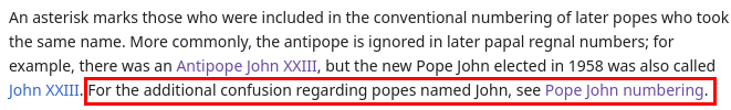
The Wikipedia article on antipopes can be pretty confusing! If you’d like to be even more confused, it can help with that!
Pages
Recent Publications
- Managing Hidden Dependencies in OO Software: a Study Based on Open Source Projects
- Open Source Communities as Liminal Ecosystems
- Investigating developers' email discussions during decision-making in Python language evolution
- Developers, Quality Control and Download Volume in Open Source Software (OSS) Projects
FLOSS Project Planets
- www-zh-cn @ Savannah: Welcome our new member - bingchuanjuzi
- Matt Glaman: Lenient Composer Plugin officially replaces lenient packages endpoint
- libtool @ Savannah: libtool-2.5.4 released [stable]
- Trey Hunner: Python Black Friday & Cyber Monday sales (2024)
- Security advisories: Drupal core - Moderately critical - Gadget chain - SA-CORE-2024-008
FLOSS Research
- Give Your Input on the State of Open Source Survey
- Open Data and Open Source AI: Charting a course to get more of both
- The Open Source Initiative and the Eclipse Foundation to Collaborate on Shaping Open Source AI (OSAI) Public Policy
- ClearlyDefined v2.0 adds support for LicenseRefs
- ClearlyDefined at SOSS Fusion 2024: a collaborative solution to Open Source license compliance