
Feeds
Drupal Association blog: Drupal Innovation in 2024: the Contribution Health Dashboards
2023 has been an eventful year, full of ideas, discussions and plans regarding innovation, where Drupal is heading, and, in our case, how the Drupal Association can best support. On top of that, you may have already heard, but innovation is a key goal for the Drupal Association.
Drupal is nothing but a big, decentralized, community. And before we can even think of how we can innovate, we need to understand how contribution actually happens and evolves in our ecosystem. And one of the things we agreed early on was that, without numbers, we don’t even know where we are going.
For that reason in 2024 we want to introduce you to part of the work we’ve been doing during the last part of 2023 to make sure that we know where we are coming from, we understand where we are going and how the changes we are doing are affecting (or not) the whole contribution ecosystem. I want to introduce you to the Contribution Health Dashboards (CHD).
The CH dashboards should help identify what stops or blocks people from contributing, uncover any friction, and if any problems are found, help to investigate and apply adequate remedies while we can as well measure those changes.
One thing to note is that the numbers we are showing next are based on the contribution credit system. The credit system has been very successful in standardizing and measuring contributions to Drupal. It also provides incentives to contribute to Drupal, and has raised interest from individuals and organizations.
Using the credit system to evaluate the contribution is not 100% perfect, and it could show some flaws and imperfections, but we are committed to review and improve those indicators regularly, and we think it’s the most accurate way to measure the way contribution happens in Drupal.
It must be noted as well that the data is hidden, deep, in the Drupal.org database. Extracting that data has proved a tedious task, and there are numbers and statistics that we would love to extract in the near future to validate further the steps we are taking. Again, future reviews of the work will happen during the next months while we continue helping contributors to continue innovating.
You can find the dashboards here, in the Contribution Health Dashboards, but keep reading next to understand the numbers better.
Unique individuals and organisationsJumping to what matters here, the numbers, one of the most important metrics to understand in the Drupal ecosystem is the number of contributions of both individuals and organisations.
As you can see, the number of individuals has stayed relatively stable, while their contribution has been more and more significant over the years (except for a slide in the first year of the pandemic). In a way this is telling us that once a user becomes a contributor, they stay for the long run. And, in my opinion, the numbers say that they stay actually very committed.
The number of organisations on the other hand displays a growing healthy trend. This shows that organisations are an important partner for Drupal and the Drupal Association, bringing a lot of value in the form of (but not just) contributors.
It definitely means that we need to continue supporting and listening to them. It’s actually a symbiotic relationship. These companies support and help moving forward, not just Drupal, but the whole concept of the Open Web. And their involvement doesn’t end up there, as their daily role in expanding the reach, the number of instances and customers of every size using Drupal is as well key.
In practical terms in 2023 we have been meeting different companies and organisations, and the plan is to continue listening and finding new ways to help their needs in 2024 and beyond. One of the things we are releasing soon is the list of priorities and strategic initiatives where your contributions, as individuals as well as organisations, are most meaningful. This is something I have been consistently asked for when meeting with those individuals and organisations, and I think it’s going to make a big difference unleashing innovation in Drupal. I recommend you to have a look at the blog post about the bounty program.
First year contributorsThe next value we should be tracking is how first time users are interacting with our ecosystem.
While the previous numbers are encouraging, we have a healthy ecosystem of companies and a crowd of loyal individuals contributing to the project, making sure that we onboard and we make it easier and attractive for new generations to contribute to the project is the only possible way to ensure that this continues to be the case for many years to come.
That’s why we are looking at first time contributions, or said differently, how many users make a first contribution in their first 12 months from joining the project. During 2024 I would like to look deeper into this data, reveal contribution data further on time, like after 24 and 36 months. For now this will be a good lighthouse that we can use to improve the contribution process.
Although last year's numbers give us a nice feeling of success, we want to be cautious about them, and try to make sure that the trend of previous years of a slight decline does not continue.
That is the reason why my first priority during the first months of 2024 is to review the registration process and the next step for new users on their contribution journey. From the form they are presented, to the documentation we are facilitating, to the messages we are sending them in the weeks and months after.
The changes we make should be guided as well by the next important graph, which is the Time To First Contribution. In other words, the amount of time a new user has taken to make their first contribution to Drupal.
You’ll see that the Contribution Health Dashboards includes other data that I have not mentioned in this post. It does not mean that it is not equally important, but given the Drupal Association has a finite amount of resources, we consider that this is the data that we need to track closely to get a grasp of the health of our contribution system.
For now, have a look at the Contribution Health Dashboards to get a grasp of the rest of the information that we have collected. If you are curious about the numbers and maybe would like to give us a hand, please do not hesitate to send me a message at alex.moreno@association.drupal.org
PyCon: Applications For Booth Space on Startup Row Are Now Open!
Applications For Booth Space on Startup Row Are Now Open
To all the startup founders out there, PyCon US organizers have some awesome news for you! The application window for Startup Row at PyCon US is now open.
You’ve got until March 15th to apply, but don’t delay. (And if you want to skip all this reading and go straight to the application, here’s a link for ya.)
That’s right! Your startup could get the best of what PyCon US has to offer:
- Coveted Expo Hall booth space
- Exclusive placement on the PyCon US website
- Access to the PyCon Jobs Fair (since, after all, there’s no better place to meet and recruit Python professionals)
- A unique in-person platform to access a fantastically diverse crowd of thousands of engineers, data wranglers, academic researchers, students, and enthusiasts who come to PyCon US.
Corporate sponsors pay thousands of dollars for this level of access, but to support the entrepreneurial community PyCon US organizers are excited to give the PyCon experience to up-and-coming startup companies for free. (Submitting a Startup Row application is completely free. To discourage no-shows at the conference itself, we do require a fully-refundable $400 deposit from companies who are selected for and accept a spot on Startup Row. If you show up, you’ll get your deposit back after the conference.)
Does My Startup Qualify?The goal of Startup Row is to give seed and early-stage companies access to the Python community. Here are the qualification criteria:
- Somewhat obviously: Python is used somewhere in your tech or business stack, the more of it the better!
- Your startup is roughly 2.5 years or less at the time of applying. (If you had a major pivot or took awhile to get a product in the market, measure from there.)
- You have 25 or fewer folks on the team, including founders, employees, and contractors.
- You or your company will fund travel and accommodation to PyCon US 2024 in Pittsburgh, Pennsylvania. (There’s a helpful page on the PyCon US website with venue and hotel information.)
- You haven’t already presented on Startup Row or sponsored a previous PyCon US. (If you applied before but weren’t accepted, please do apply again!)
There is a little bit of wiggle room. If your startup is more of a fuzzy rather than an exact match for these criteria, still consider applying.
How Do I Apply?Assuming you’ve already created a user account on the PyCon US website, applying for Startup Row is easy.
- Make sure you’re logged in.
- Go to the Startup Row application page and submit your application by March 15th. (Note: It might be helpful to draft your answers in a separate document.)
- Wait to hear back! Our goal is to notify folks about their application decision toward the end of March.
Again, the application deadline is March 15, 2024 at 11:59 PM Eastern. Applications submitted after that deadline may not be considered.
Can I learn more about Startup Row?You bet! Check out the Startup Row page for more details and testimonials from prior Startup Row participants. (There’s a link to the application there, too!)
Who do I contact with questions about Startup Row?First off, if you have questions about PyCon US in general, you can send an email to the PyCon US organizing team at pycon-reg@python.org. We’re always happy to help.
For specific Startup Row-related questions, reach out to co-chair Jason D. Rowley via email at jdr [at] omg [dot] lol, or find some time in his calendar at calendly [dot] com [slash] jdr.
Wait, What’s The Deadline Again?Again, the application deadline is March 15, 2024 at 11:59PM Eastern.
Good luck! We look forward to reviewing your application!
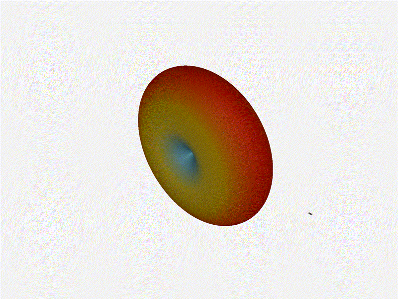
Paul Tagliamonte: Writing a simulator to check phased array beamforming 🌀
If you're on the Fediverse, I'd very much appreciate boosts on my toot!
While working on hz.tools, I started to move my beamforming code from 2-D (meaning, beamforming to some specific angle on the X-Y plane for waves on the X-Y plane) to 3-D. I’ll have more to say about that once I get around to publishing the code as soon as I’m sure it’s not completely wrong, but in the meantime I decided to write a simple simulator to visually check the beamformer against the textbooks. The results were pretty rad, so I figured I’d throw together a post since it’s interesting all on its own outside of beamforming as a general topic.
I figured I’d write this in Rust, since I’ve been using Rust as my primary language over at zoo, and it’s a good chance to learn the language better.
⚠️ This post has some large GIFsIt make take a little bit to load depending on your internet connection. Sorry about that, I'm not clever enough to do better without doing tons of complex engineering work. They may be choppy while they load or something. I tried to compress an ensmall them, so if they're loaded but fuzzy, click on them to load a slightly larger version.
This post won’t cover the basics of how phased arrays work or the specifics of calculating the phase offsets for each antenna, but I’ll dig into how I wrote a simple “simulator” and how I wound up checking my phase offsets to generate the renders below.
AssumptionsI didn’t want to build a general purpose RF simulator, anything particularly generic, or something that would solve for any more than the things right in front of me. To do this as simply (and quickly – all this code took about a day to write, including the beamforming math) – I had to reduce the amount of work in front of me.
Given that I was concerend with visualizing what the antenna pattern would look like in 3-D given some antenna geometry, operating frequency and configured beam, I made the following assumptions:
All anetnnas are perfectly isotropic – they receive a signal that is exactly the same strength no matter what direction the signal originates from.
There’s a single point-source isotropic emitter in the far-field (I modeled this as being 1 million meters away – 1000 kilometers) of the antenna system.
There is no noise, multipath, loss or distortion in the signal as it travels through space.
Antennas will never interfere with each other.
2-D Polar PlotsThe last time I wrote something like this, I generated 2-D GIFs which show a radiation pattern, not unlike the polar plots you’d see on a microphone.
These are handy because it lets you visualize what the directionality of the antenna looks like, as well as in what direction emissions are captured, and in what directions emissions are nulled out. You can see these plots on spec sheets for antennas in both 2-D and 3-D form.
Now, let’s port the 2-D approach to 3-D and see how well it works out.
Writing the 3-D simulatorAs an EM wave travels through free space, the place at which you sample the wave controls that phase you observe at each time-step. This means, assuming perfectly synchronized clocks, a transmitter and receiver exactly one RF wavelength apart will observe a signal in-phase, but a transmitter and receiver a half wavelength apart will observe a signal 180 degrees out of phase.
This means that if we take the distance between our point-source and antenna element, divide it by the wavelength, we can use the fractional part of the resulting number to determine the phase observed. If we multiply that number (in the range of 0 to just under 1) by tau, we can generate a complex number by taking the cos and sin of the multiplied phase (in the range of 0 to tau), assuming the transmitter is emitting a carrier wave at a static amplitude and all clocks are in perfect sync.
let observed_phases: Vec<Complex> = antennas .iter() .map(|antenna| { let distance = (antenna - tx).magnitude(); let distance = distance - (distance as i64 as f64); ((distance / wavelength) * TAU) }) .map(|phase| Complex(phase.cos(), phase.sin())) .collect();At this point, given some synthetic transmission point and each antenna, we know what the expected complex sample would be at each antenna. At this point, we can adjust the phase of each antenna according to the beamforming phase offset configuration, and add up every sample in order to determine what the entire system would collectively produce a sample as.
let beamformed_phases: Vec<Complex> = ...; let magnitude = beamformed_phases .iter() .zip(observed_phases.iter()) .map(|(beamformed, observed)| observed * beamformed) .reduce(|acc, el| acc + el) .unwrap() .abs();Armed with this information, it’s straight forward to generate some number of (Azimuth, Elevation) points to sample, generate a transmission point far away in that direction, resolve what the resulting Complex sample would be, take its magnitude, and use that to create an (x, y, z) point at (azimuth, elevation, magnitude). The color attached two that point is based on its distance from (0, 0, 0). I opted to use the Life Aquatic table for this one.
After this process is complete, I have a point cloud of ((x, y, z), (r, g, b)) points. I wrote a small program using kiss3d to render point cloud using tons of small spheres, and write out the frames to a set of PNGs, which get compiled into a GIF.
Now for the fun part, let’s take a look at some radiation patterns!
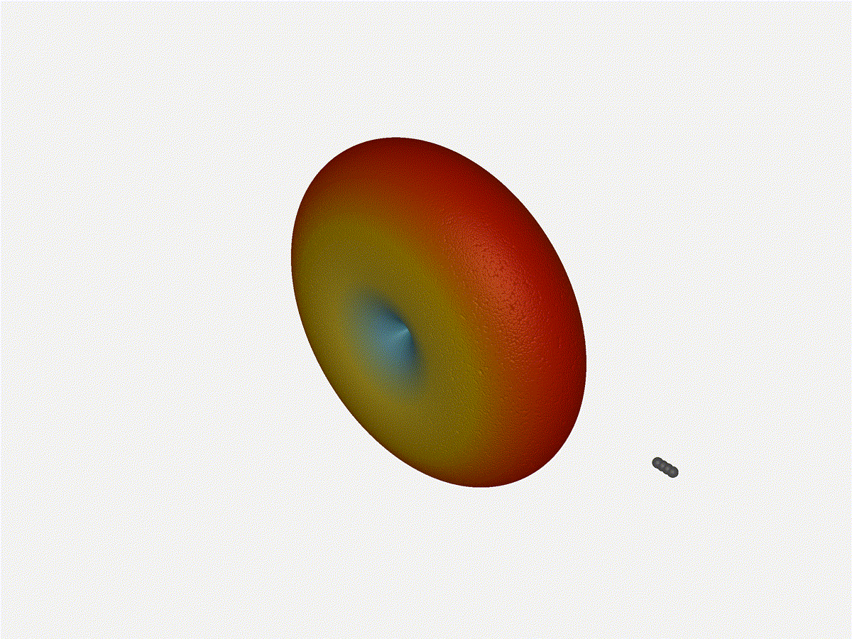
1x4 Phased ArrayThe first configuration is a phased array where all the elements are in perfect alignment on the y and z axis, and separated by some offset in the x axis. This configuration can sweep 180 degrees (not the full 360), but can’t be steared in elevation at all.
Let’s take a look at what this looks like for a well constructed 1x4 phased array:
And now let’s take a look at the renders as we play with the configuration of this array and make sure things look right. Our initial quarter-wavelength spacing is very effective and has some outstanding performance characteristics. Let’s check to see that everything looks right as a first test.
Nice. Looks perfect. When pointing forward at (0, 0), we’d expect to see a torus, which we do. As we sweep between 0 and 360, astute observers will notice the pattern is mirrored along the axis of the antennas, when the beam is facing forward to 0 degrees, it’ll also receive at 180 degrees just as strong. There’s a small sidelobe that forms when it’s configured along the array, but it also becomes the most directional, and the sidelobes remain fairly small.
Long compared to the wavelength (1¼ λ)Let’s try again, but rather than spacing each antenna ¼ of a wavelength apart, let’s see about spacing each antenna 1¼ of a wavelength apart instead.
The main lobe is a lot more narrow (not a bad thing!), but some significant sidelobes have formed (not ideal). This can cause a lot of confusion when doing things that require a lot of directional resolution unless they’re compensated for.
Going from (¼ to 5¼ λ)The last model begs the question - what do things look like when you separate the antennas from each other but without moving the beam? Let’s simulate moving our antennas but not adjusting the configured beam or operating frequency.
Very cool. As the spacing becomes longer in relation to the operating frequency, we can see the sidelobes start to form out of the end of the antenna system.
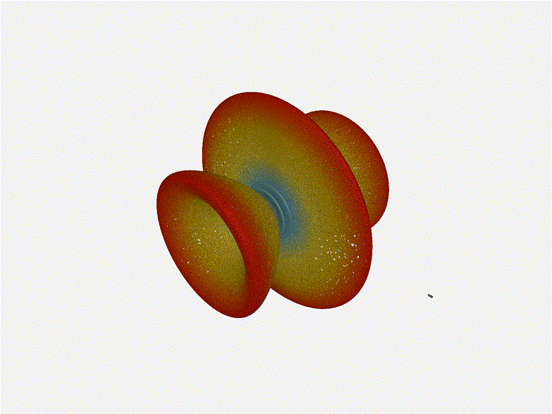
2x2 Phased ArrayThe second configuration I want to try is a phased array where the elements are in perfect alignment on the z axis, and separated by a fixed offset in either the x or y axis by their neighbor, forming a square when viewed along the x/y axis.
Let’s take a look at what this looks like for a well constructed 2x2 phased array:
Let’s do the same as above and take a look at the renders as we play with the configuration of this array and see what things look like. This configuration should suppress the sidelobes and give us good performance, and even give us some amount of control in elevation while we’re at it.
Sweet. Heck yeah. The array is quite directional in the configured direction, and can even sweep a little bit in elevation, a definite improvement from the 1x4 above.
Long compared to the wavelength (1¼ λ)Let’s do the same thing as the 1x4 and take a look at what happens when the distance between elements is long compared to the frequency of operation – say, 1¼ of a wavelength apart? What happens to the sidelobes given this spacing when the frequency of operation is much different than the physical geometry?
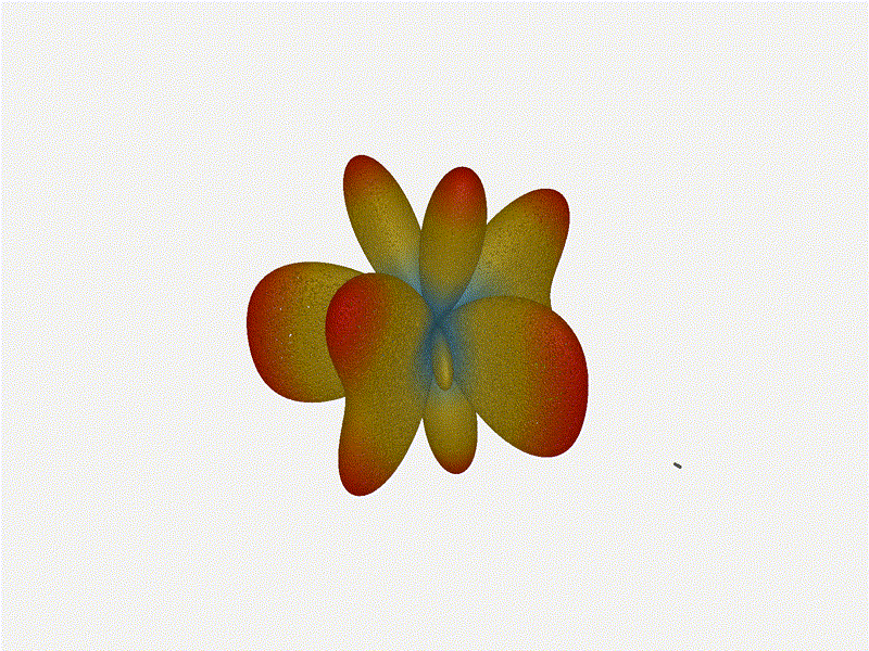
Mesmerising. This is my favorate render. The sidelobes are very fun to watch come in and out of existence. It looks absolutely other-worldly.
Going from (¼ to 5¼ λ)Finally, for completeness' sake, what do things look like when you separate the antennas from each other just as we did with the 1x4? Let’s simulate moving our antennas but not adjusting the configured beam or operating frequency.
Very very cool. The sidelobes wind up turning the very blobby cardioid into an electromagnetic dog toy. I think we’ve proven to ourselves that using a phased array much outside its designed frequency of operation seems like a real bad idea.
Future WorkNow that I have a system to test things out, I’m a bit more confident that my beamforming code is close to right! I’d love to push that code over the line and blog about it, since it’s a really interesting topic on its own. Once I’m sure the code involved isn’t full of lies, I’ll put it up on the hztools org, and post about it here and on mastodon.
Real Python: When to Use a List Comprehension in Python
One of Python’s most distinctive features is the list comprehension, which you can use to create powerful functionality within a single line of code. However, many developers struggle to fully leverage the more advanced features of list comprehensions in Python. Some programmers even use them too much, which can lead to code that’s less efficient and harder to read.
By the end of this tutorial, you’ll understand the full power of Python list comprehensions and know how to use their features comfortably. You’ll also gain an understanding of the trade-offs that come with using them so that you can determine when other approaches are preferable.
In this tutorial, you’ll learn how to:
- Rewrite loops and map() calls as list comprehensions in Python
- Choose between comprehensions, loops, and map() calls
- Supercharge your comprehensions with conditional logic
- Use comprehensions to replace filter()
- Profile your code to resolve performance questions
Get Your Code: Click here to download the free code that shows you how and when to use list comprehensions in Python.
Transforming Lists in PythonThere are a few different ways to create and add items to a lists in Python. In this section, you’ll explore for loops and the map() function to perform these tasks. Then, you’ll move on to learn about how to use list comprehensions and when list comprehensions can benefit your Python program.
Use for LoopsThe most common type of loop is the for loop. You can use a for loop to create a list of elements in three steps:
- Instantiate an empty list.
- Loop over an iterable or range of elements.
- Append each element to the end of the list.
If you want to create a list containing the first ten perfect squares, then you can complete these steps in three lines of code:
Python >>> squares = [] >>> for number in range(10): ... squares.append(number * number) ... >>> squares [0, 1, 4, 9, 16, 25, 36, 49, 64, 81] Copied!Here, you instantiate an empty list, squares. Then, you use a for loop to iterate over range(10). Finally, you multiply each number by itself and append the result to the end of the list.
Work With map ObjectsFor an alternative approach that’s based in functional programming, you can use map(). You pass in a function and an iterable, and map() will create an object. This object contains the result that you’d get from running each iterable element through the supplied function.
As an example, consider a situation in which you need to calculate the price after tax for a list of transactions:
Python >>> prices = [1.09, 23.56, 57.84, 4.56, 6.78] >>> TAX_RATE = .08 >>> def get_price_with_tax(price): ... return price * (1 + TAX_RATE) ... >>> final_prices = map(get_price_with_tax, prices) >>> final_prices <map object at 0x7f34da341f90> >>> list(final_prices) [1.1772000000000002, 25.4448, 62.467200000000005, 4.9248, 7.322400000000001] Copied!Here, you have an iterable, prices, and a function, get_price_with_tax(). You pass both of these arguments to map() and store the resulting map object in final_prices. Finally, you convert final_prices into a list using list().
Leverage List ComprehensionsList comprehensions are a third way of making or transforming lists. With this elegant approach, you could rewrite the for loop from the first example in just a single line of code:
Python >>> squares = [number * number for number in range(10)] >>> squares [0, 1, 4, 9, 16, 25, 36, 49, 64, 81] Copied!Rather than creating an empty list and adding each element to the end, you simply define the list and its contents at the same time by following this format:
new_list = [expression for member in iterable]Every list comprehension in Python includes three elements:
- expression is the member itself, a call to a method, or any other valid expression that returns a value. In the example above, the expression number * number is the square of the member value.
- member is the object or value in the list or iterable. In the example above, the member value is number.
- iterable is a list, set, sequence, generator, or any other object that can return its elements one at a time. In the example above, the iterable is range(10).
[ Improve Your Python With 🐍 Python Tricks 💌 – Get a short & sweet Python Trick delivered to your inbox every couple of days. >> Click here to learn more and see examples ]
Russell Coker: Storage Trends 2024
It has been less than a year since my last post about storage trends [1] and enough has changed to make it worth writing again. My previous analysis was that for <2TB only SSD made sense, for 4TB SSD made sense for business use while hard drives were still a good option for home use, and for 8TB+ hard drives were clearly the best choice for most uses. I will start by looking at MSY prices, they aren't the cheapest (you can get cheaper online) but they are competitive and they make it easy to compare the different options. I'll also compare the cheapest options in each size, there are more expensive options but usually if you want to pay more then the performance benefits of SSD (both SATA and NVMe) are even more appealing. All prices are in Australian dollars and of parts that are readily available in Australia, but the relative prices of the parts are probably similar in most countries. The main issue here is when to use SSD and when to use hard disks, and then if SSD is chosen which variety to use.
Small StorageFor my last post the cheapest storage devices from MSY were $19 for a 128G SSD, now it’s $24 for a 128G SSD or NVMe device. I don’t think the Australian dollar has dropped much against foreign currencies, so I guess this is partly companies wanting more profits and partly due to the demand for more storage. Items that can’t sell in quantity need higher profit margins if they are to have them in stock. 500G SSDs are around $33 and 500G NVMe devices for $36 so for most use cases it wouldn’t make sense to buy anything smaller than 500G.
The cheapest hard drive is $45 for a 1TB disk. A 1TB SATA SSD costs $61 and a 1TB NVMe costs $79. So 1TB disks aren’t a good option for any use case.
A 2TB hard drive is $89. A 2TB SATA SSD is $118 and a 2TB NVMe is $145. I don’t think the small savings you can get from using hard drives makes them worth using for 2TB.
For most people if you have a system that’s important to you then $145 on storage isn’t a lot to spend. It seems hardly worth buying less than 2TB of storage, even for a laptop. Even if you don’t use all the space larger storage devices tend to support more writes before wearing out so you still gain from it. A 2TB NVMe device you buy for a laptop now could be used in every replacement laptop for the next 10 years. I only have 512G of storage in my laptop because I have a collection of SSD/NVMe devices that have been replaced in larger systems, so the 512G is essentially free for my laptop as I bought a larger device for a server.
For small business use it doesn’t make sense to buy anything smaller than 2TB for any system other than a router. If you buy smaller devices then you will sometimes have to pay people to install bigger ones and when the price is $145 it’s best to just pay that up front and be done with it.
Medium StorageA 4TB hard drive is $135. A 4TB SATA SSD is $319 and a 4TB NVMe is $299. The prices haven’t changed a lot since last year, but a small increase in hard drive prices and a small decrease in SSD prices makes SSD more appealing for this market segment.
A common size range for home servers and small business servers is 4TB or 8TB of storage. To do that on SSD means about $600 for 4TB of RAID-1 or $900 for 8TB of RAID-5/RAID-Z. That’s quite affordable for that use.
For 8TB of less important storage a 8TB hard drive costs $239 and a 8TB SATA SSD costs $899 so a hard drive clearly wins for the specific case of non-RAID single device storage. Note that the U.2 devices are more competitive for 8TB than SATA but I included them in the next section because they are more difficult to install.
Serious StorageWith 8TB being an uncommon and expensive option for consumer SSDs the cheapest price is for multiple 4TB devices. To have multiple NVMe devices in one PCIe slot you need PCIe bifurcation (treating the PCIe slot as multiple slots). Most of the machines I use don’t support bifurcation and most affordable systems with ECC RAM don’t have it. For cheap NVMe type storage there are U.2 devices (the “enterprise” form of NVMe). Until recently they were too expensive to use for desktop systems but now there are PCIe cards for internal U.2 devices, $14 for a card that takes a single U.2 is a common price on AliExpress and prices below $600 for a 7.68TB U.2 device are common – that’s cheaper on a per-TB basis than SATA SSD and NVMe! There are PCIe cards that take up to 4*U.2 devices (which probably require bifurcation) which means you could have 8+ U.2 devices in one not particularly high end PC for 56TB of RAID-Z NVMe storage. Admittedly $4200 for 56TB is moderately expensive, but it’s in the price range for a small business server or a high end home server. A more common configuration might be 2*7.68TB U.2 on a single PCIe card (or 2 cards if you don’t have bifurcation) for 7.68TB of RAID-1 storage.
For SATA SSD AliExpress has a 6*2.5″ hot-swap device that fits in a 5.25″ bay for $63, so if you have 2*5.25″ bays you could have 12*4TB SSDs for 44TB of RAID-Z storage. That wouldn’t be much cheaper than 8*7.68TB U.2 devices and would be slower and have less space. But it would be a good option if PCIe bifurcation isn’t possible.
16TB SATA hard drives cost $559 which is almost exactly half the price per TB of U.2 storage. That doesn’t seem like a good deal. If you want 16TB of RAID storage then 3*7.68TB U.2 devices only costs about 50% more than 2*16TB SATA disks. In most cases paying 50% more to get NVMe instead of hard disks is a good option. As sizes go above 16TB prices go up in a more than linear manner, I guess they don’t sell much volume of larger drives.
15.36TB U.2 devices are on sale for about $1300, slightly more than twice the price of a 16TB disk. It’s within the price range of small businesses and serious home users. Also it should be noted that the U.2 devices are designed for “enterprise” levels of reliability and the hard disk prices I’m comparing to are the cheapest available. If “NAS” hard disks were compared then the price benefit of hard disks would be smaller.
Probably the biggest problem with U.2 for most people is that it’s an uncommon technology that few people have much experience with or spare parts for testing. Also you can’t buy U.2 gear at your local computer store which might mean that you want to have spare parts on hand which is an extra expense.
For enterprise use I’ve recently been involved in discussions with a vendor that sells multiple petabyte arrays of NVMe. Apparently NVMe is cheap enough that there’s no need to use anything else if you want a well performing file server.
Do Hard Disks Make Sense?There are specific cases like comparing a 8TB hard disk to a 8TB SATA SSD or a 16TB hard disk to a 15.36TB U.2 device where hard disks have an apparent advantage. But when comparing RAID storage and counting the performance benefits of SSD the savings of using hard disks don’t seem to be that great.
Is now the time that hard disks are going to die in the market? If they can’t get volume sales then prices will go up due to lack of economy of scale in manufacture and increased stock time for retailers. 8TB hard drives are now more expensive than they were 9 months ago when I wrote my previous post, has a hard drive price death spiral already started?
SSDs are cheaper than hard disks at the smallest sizes, faster (apart from some corner cases with contiguous IO), take less space in a computer, and make less noise. At worst they are a bit over twice the cost per TB. But the most common requirements for storage are small enough and cheap enough that being twice as expensive as hard drives isn’t a problem for most people.
I predict that hard disks will become less popular in future and offer less of a price advantage. The vendors are talking about 50TB hard disks being available in future but right now you can fit more than 50TB of NVMe or U.2 devices in a volume less than that of a 3.5″ hard disk so for storage density SSD can clearly win. Maybe in future hard disks will be used in arrays of 100TB devices for large scale enterprise storage. But for home users and small businesses the current sizes of SSD cover most uses.
At the moment it seems that the one case where hard disks can really compare well is for backup devices. For backups you want large storage, good contiguous write speeds, and low prices so you can buy plenty of them.
Further IssuesThe prices I’ve compared for SATA SSD and NVMe devices are all based on the cheapest devices available. I think it’s a bit of a market for lemons [2] as devices often don’t perform as well as expected and the incidence of fake products purporting to be from reputable companies is high on the cheaper sites. So you might as well buy the cheaper devices. An advantage of the U.2 devices is that you know that they will be reliable and perform well.
One thing that concerns me about SSDs is the lack of knowledge of their failure cases. Filesystems like ZFS were specifically designed to cope with common failure cases of hard disks and I don’t think we have that much knowledge about how SSDs fail. But with 3 copies of metadata BTFS or ZFS should survive unexpected SSD failure modes.
I still have some hard drives in my home server, they keep working well enough and the prices on SSDs keep dropping. But if I was buying new storage for such a server now I’d get U.2.
I wonder if tape will make a comeback for backup.
Does anyone know of other good storage options that I missed?
- [1] https://etbe.coker.com.au/2023/04/09/storage-trends-2023/
- [2] https://en.wikipedia.org/wiki/The_Market_for_Lemons
Related posts:
- Storage Trends 2023 It’s been 2 years since my last blog post about...
- Storage Trends 2021 The Viability of Small Disks Less than a year ago...
- Storage Trends In considering storage trends for the consumer side I’m looking...
LN Webworks: AWS S3 Bucket File Upload In Drupal
- Log in to AWS Console: Go to the AWS Management Console and log in to your account.
- Navigate to S3: In the AWS Console, find and click on the "S3" service.
- Create a Bucket: Click the "Create bucket" button, provide a unique and meaningful name for your bucket, and choose the region where you want to create the bucket.
- Configure Options: Set the desired configuration options, such as versioning, logging, and tags. Click through the configuration steps, review your settings, and create the bucket.
$settings['s3fs.access_key'] = "YOUR_ACCESS_KEY";
$settings['s3fs.secret_key'] = "YOUR_SECRET_KEY";
$settings['s3fs.region'] = "us-east-1";
$settings['s3fs.upload_as_public'] = TRUE;
ADCI Solutions: How to Upgrade Drupal 7 and 8 to Drupal 10: Step-by-Step Guide
Developers of the ADCI Solutions Studio explain why you need to upgrade your Drupal 7 and 8 websites to Drupal 10 and what makes the migration process different from a routine CMS update.
Zato Blog: How to correctly integrate APIs in Python
Understanding how to effectively integrate various systems and APIs is crucial. Yet, without a dedicated integration platform, the result will be brittle point-to-point integrations that never lead to good outcomes.
➤ Read this article about Zato, an open-source integration platform in Python, for an overview of what to avoid and how to do it correctly instead.
More blog posts➤Dirk Eddelbuettel: RProtoBuf 0.4.22 on CRAN: Updated Windows Support!
A new maintenance release 0.4.22 of RProtoBuf arrived on CRAN earlier today. RProtoBuf provides R with bindings for the Google Protocol Buffers (“ProtoBuf”) data encoding and serialization library used and released by Google, and deployed very widely in numerous projects as a language and operating-system agnostic protocol.
This release matches the recent 0.4.21 release which enabled use of the package with newer ProtoBuf releases. Tomas has been updating the Windows / rtools side of things, and supplied us with simple PR that will enable building with those updated versions once finalised.
The following section from the NEWS.Rd file has full details.
Changes in RProtoBuf version 0.4.22 (2022-12-13)- Apply patch by Tomas Kalibera to support updated rtools to build with newer ProtoBuf releases on windows
Thanks to my CRANberries, there is a diff to the previous release. The RProtoBuf page has copies of the (older) package vignette, the ‘quick’ overview vignette, and the pre-print of our JSS paper. Questions, comments etc should go to the GitHub issue tracker off the GitHub repo.
If you like this or other open-source work I do, you can sponsor me at GitHub.
This post by Dirk Eddelbuettel originated on his Thinking inside the box blog. Please report excessive re-aggregation in third-party for-profit settings.
Luke Plant: Python packaging must be getting better - a datapoint
I’m developing some Python software for a client, which in its current early state is desktop software that will need to run on Windows.
So far, however, I have done all development on my normal comfortable Linux machine. I haven’t really used Windows in earnest for more than 15 years – to the point where my wife happily installs Linux on her own machine, knowing that I’ll be hopeless at helping her fix issues if the OS is Windows – and certainly not for development work in that time. So I was expecting a fair amount of pain.
There was certainly a lot of friction getting a development environment set up. RealPython.com have a great guide which got me a long way, but even that had some holes and a lot of inconvenience, mostly due to the fact that, on the machine I needed to use, my main login and my admin login are separate. (I’m very lucky to be granted an admin login at all, so I’m not complaining). And there are lots of ways that Windows just seems to be broken, but that’s another blog post.
When it came to getting my app running, however, I was very pleasantly surprised.
At this stage in development, I just have a rough requirements.txt that I add Python deps to manually. This might be a good thing, as I avoid the pain of some the additional layers people have added.
So after installing Python and creating a virtual environment on Windows, I ran pip install -r requirements.txt, expecting a world of pain, especially as I already had complex non-Python dependencies, including Qt5 and VTK. I had specified both of these as simple Python deps via the wrappers pyqt5 and vtk in my requirements.txt, and nothing else, with the attitude of “well I may as well dream this is going to work”.
And in fact, it did! Everything just downloaded as binary wheels – rather large ones, but that’s fine. I didn’t need compilers or QMake or header files or anything.
And when I ran my app, apart from a dependency that I’d forgotten to add to requirements.txt, everything worked perfectly first time. This was even more surprising as I had put zero conscious effort into Windows compatibility. In retrospect I realise that use of pathlib, which is automatic for me these days, had helped me because it smooths over some Windows/Unix differences with path handling.
Of course, this is a single datapoint. From other people’s reports there are many, many ways that this experience may not be typical. But that it is possible at all suggests that a lot of progress has been made and we are very much going in the right direction. A lot of people have put a lot of work in to achieve that, for which I’m very grateful!
Debian Brasil: MiniDebConf BH 2024 - patrocínio e financiamento coletivo
Já está rolando a inscrição de participante e a chamada de atividades para a MiniDebConf Belo Horizonte 2024, que acontecerá de 27 a 30 de abril no Campus Pampulha da UFMG.
Este ano estamos ofertando bolsas de alimentação, hospedagem e passagens para contribuidores(as) ativos(as) do Projeto Debian.
Patrocínio:Para a realização da MiniDebConf, estamos buscando patrocínio financeiro de empresas e entidades. Então se você trabalha em uma empresa/entidade (ou conhece alguém que trabalha em uma) indique o nosso plano de patrocínio para ela. Lá você verá os valores de cada cota e os seus benefícios.
Financiamento coletivo:Mas você também pode ajudar a realização da MiniDebConf por meio do nosso financiamento coletivo!
Faça uma doação de qualquer valor e tenha o seu nome publicado no site do evento como apoiador(a) da MiniDebConf Belo Horizonte 2024.
Mesmo que você não pretenda vir a Belo Horizonte para participar do evento, você pode doar e assim contribuir para o mais importante evento do Projeto Debian no Brasil.
ContatoQualquer dúvida, mande um email para contato@debianbrasil.org.br
OrganizaçãoTechBeamers Python: LangChain Agent Basics with Sample Agent Code
LangChain agents are fascinating creatures! They live in the world of text and code, interacting with humans through conversations and completing tasks based on instructions. Think of them as your digital assistants, but powered by artificial intelligence and fueled by language models. Getting Started with Agents in LangChain Imagine a chatty robot friend that gets […]
The post LangChain Agent Basics with Sample Agent Code appeared first on TechBeamers.
TechBeamers Python: LangChain Memory Basics
Langchain Memory is like a brain for your conversational agents. It remembers past chats, making conversations flow smoothly and feel more personal. Think of it like chatting with a real friend who recalls what you talked about before. This makes the agent seem smarter and more helpful. Getting Started with Memory in LangChain Imagine you’re […]
The post LangChain Memory Basics appeared first on TechBeamers.
TypeThePipe: Data Engineering Bootcamp 2024 (Week 1) Docker & Terraform
I’ve just enrolled in the DataTalks free Data Engineering zootcamp. It’s a fantastic initiative that has been running for several years, with each cohort occurring annually.
The course is organized weekly, featuring one online session per week. There are optional weekly homework assignments which are reviewed, and the course concludes with a mandatory Data Eng final project, which is required to earn the certification.
In this series of posts, I will be sharing with you my course notes and comments, and also how I’m resolving the homework.
Let’s delve into the essentials of Docker, Dockerfile, and Docker Compose. These three components are crucial in the world of software development, especially when dealing with application deployment and management.
Docker: The Cornerstone of Containerization
Docker stands at the forefront of containerization technology. It allows developers to package applications and their dependencies into containers. A container is an isolated environment, akin to a lightweight, standalone, and secure package of software that includes everything needed to run it: code, runtime, system tools, system libraries, and settings. This technology ensures consistency across multiple development and release cycles, standardizing your environment across different stages.
Dockerfile: Blueprint for Docker images
A Dockerfile is a text document containing all the commands a user could call on the command line to assemble a Docker image. It automates the process of creating Docker images. A Dockerfile defines what goes on in the environment inside your container. It allows you to create a container that meets your specific needs, which can then be run on any Docker-enabled machine.
Docker Compose: Simplifying multi-container applications
Docker Compose is a tool for defining and running multi-container Docker applications. With Compose, you use a YAML file to configure your application’s services, networks, and volumes. Then, with a single command, you create and start all the services from your configuration. Docker Compose works in all environments: production, staging, development, testing, as well as CI workflows.
Why these tools matter?
The combination of Docker, Dockerfile, and Docker Compose streamlines the process of developing, shipping, and running applications. Docker encapsulates your application and its environment, Dockerfile builds the image for this environment, and Docker Compose manages the orchestration of multi-container setups. Together, they provide a robust and efficient way to handle the lifecycle of applications. This ecosystem is integral for developers looking to leverage the benefits of containerization for more reliable, scalable, and collaborative software development.
Get Docker and read there the documentation.
Alright, data engineers, gather around! Why should you care about containerization and Docker? Well, it’s like having a Swiss Army knife in your tech toolkit. Here’s why:
Local Experimentation: Setting up things locally for experiments becomes a breeze. No more wrestling with conflicting dependencies or environments. Docker keeps it clean and easy.
Testing and CI Made Simple: Integration tests and CI/CD pipelines? Docker smoothens these processes. It’s like having a rehearsal space for your code before it hits the big stage.
Batch Jobs and Beyond: While Docker plays nice with AWS Batch, Kubernetes jobs, and more (though that’s a story for another day), it’s a glimpse into the world of possibilities with containerization.
Spark Joy: If you’re working with Spark, Docker can be a game-changer. It’s like having a consistent and controlled playground for your data processing.
Serverless, Stress-less: With the rise of serverless architectures like AWS Lambda, Docker ensures that you’re developing in an environment that mirrors your production setup. No more surprises!
So, there you have it. Containers are everywhere, and Docker is leading the parade. It’s not just a tool; it’s an essential part of the modern software development and deployment process.
You may need to create a network in order the containers communicate. Then, run the Postgres database container. Notice that in order to persist the data, as docker containers would be stateless and reinizialized after each run, you may indicate Docker volumes to persist the PG internal and ingested data.
docker network create pg-network docker run -it \ -e POSTGRES_USER="root" \ -e POSTGRES_PASSWORD="root" \ -e POSTGRES_DB="ny_taxi" \ -v /Users/jobandtalent/data-eng-bootcamp/ny_taxi_pg_data:/var/lib/postgresql/data \ -p 5437:5432 \ --name pg-database \ --network=pg-network \ postgres:13 `` Let's create and start the PG Admin container: docker run -it \ -e PGADMIN_DEFAULT_EMAIL="admin@admin.com" \ -e PGADMIN_DEFAULT_PASSWORD="root" \ -p 8080:80 \ --name pgadmin \ --network=pg-network \ dpage/pgadmin4Instead of managing our containers individually, it is way better to manage them from one single source. The docker-compose file allows you to specify the services/containers you want to build and run, from the image to run till the environment variables and volumes.
version: "3.11" services: pg-database: image: postgres:13 environment: - POSTGRES_USER=root - POSTGRES_PASSWORD=root - POSTGRES_DB=ny_taxi volumes: - ./ny_taxi_pg_data:/var/lib/postgresql/data ports: - 5432:5432 pg-admin: image: dpage/pgadmin4 environment: - PGADMIN_DEFAULT_EMAIL=admin@admin.com - PGADMIN_DEFAULT_PASSWORD=root ports: - 8080:80 volumes: - "pgadmin_conn_data:/var/lib/pgadmin:rw" volumes: pgadmin_conn_data:The pipeline script objective is download the ddata from the US taxi rides and insert it in the Postgres database. The script could be as simple as:
import polars as pl from pydantic_settings import BaseSettings, SettingsConfigDict from typing import ClassVar TRIPS_TABLE_NAME = "green_taxi_trips" ZONES_TABLE_NAME = "zones" class PgConn(BaseSettings): model_config = SettingsConfigDict(env_prefix='PG_', env_file='.env', env_file_encoding='utf-8') user: str pwd: str host: str port: int db: str connector: ClassVar[str] = "postgresql" @property def uri(self): return f"{self.connector}://{self.user}:{self.pwd}@{self.host}:{self.port}/{self.db}" df_ny_taxi = pl.read_csv("https://github.com/DataTalksClub/nyc-tlc-data/releases/download/green/green_tripdata_2019-09.csv.gz") df_zones = pl.read_csv("https://s3.amazonaws.com/nyc-tlc/misc/taxi+_zone_lookup.csv") conn = PgConn() df_zones.write_database(ZONES_TABLE_NAME, conn.uri) df_ny_taxi.write_database(TRIPS_TABLE_NAME, conn.uri)We have used Polars and Pydantic (v2) libraries. With Polars, we load the data from csvs and also manage how to write it to the database with write_database DataFrame method. We load Pydantic module in order to create a Postgres connection object, that loads the configuration from the environment. We are using for convenience an .env config file, but it is not mandatory. As we will explain in the following chunk of code, we set the env variables on the Dockerfile and they remain accessible from inside the container, being trivial to load them using BaseSettings and SettingsConfigDict.
Now, in order to Dockerize your data pipeline script, that as we just saw it download and ingest the data to Postgres, we need to create a Dockerfile with the specifications of the container. We are using Poetry as a dependency manager, so we need to include those pyproject.toml (multi-pourpose file, used to specify to Poetry the desired module version constraints) and the poetry.lock (specific for Poetry version pin respecting the package version constraints from pyproject.toml). Also, we may include to the container the actual ingest_data.py Python pipeline file.
FROM python:3.11 ARG POETRY_VERSION=1.7.1 WORKDIR /app COPY ingest_data.py ingest_data.py COPY .env .env COPY pyproject.toml pyproject.toml COPY poetry.lock poetry.lock RUN pip3 install --no-cache-dir poetry==${POETRY_VERSION} \ && poetry env use 3.11 \ && poetry install --no-cache ENTRYPOINT [ "poetry", "run", "python", "ingest_data.py" ]Just by building the container in our root folder and running it, the ingest_data.py script will be executed, and therefore the data downloaded and persisted on the Postgres database.
Terraform has become a key tool in modern infrastructure management. Terraform, named with a nod to the concept of terraforming planets, applies a similar idea to cloud and local platform infrastructure. It’s about creating and managing the necessary environment for software to run efficiently on platforms like AWS, GCP…
Terraform, developed by HashiCorp, is described as an “infrastructure as code” tool. It allows users to define and manage both cloud-based and on-premises resources in human-readable configuration files. These files can be versioned, reused, and shared, offering a consistent workflow to manage infrastructure throughout its lifecycle. The advantages of using Terraform include simplicity in tracking and modifying infrastructure, ease of collaboration (since configurations are file-based and can be shared on platforms like GitHub), and reproducibility. For instance, an infrastructure set up in a development environment can be replicated in production with minor adjustments. Additionally, Terraform helps in ensuring that resources are properly removed when no longer needed, avoiding unnecessary costs.
So this tool not only simplifies the process of infrastructure management but also ensures consistency and compliance with your infrastructure setup.
However, it’s important to note what Terraform is not. It doesn’t handle the deployment or updating of software on the infrastructure; it’s focused solely on the infrastructure itself. It doesn’t allow modifications to immutable resources without destroying and recreating them. For example, changing the type of a virtual machine would require its recreation. Terraform also only manages resources defined within its configuration files.
Diving into the world of cloud infrastructure can be a daunting task, but with tools like Terraform, the process becomes more manageable and streamlined. Terraform, an open-source infrastructure as code software tool, allows users to define and provision a datacenter infrastructure using a high-level configuration language. Here’s a guide to setting up Terraform for Google Cloud Platform (GCP).
Creating a Service Account in GCP
Before we start coding with Terraform, it’s essential to establish a method for Terraform on our local machine to communicate with GCP. This involves setting up a service account in GCP – a special type of account used by applications, as opposed to individuals, to interact with the GCP services.
Creating a service account is straightforward. Log into the GCP console, navigate to the “IAM & Admin” section, and create a new service account. This account should be given specific permissions relevant to the resources you plan to manage with Terraform, such as Cloud Storage or BigQuery.
Once the service account is created, the next step is to manage its keys. These keys are crucial as they authenticate and authorize the Terraform script to perform actions in GCP. It’s vital to handle these keys with care, as they can be used to access your GCP resources. You should never expose these credentials publicly.
Setting Up Your Local Environment
After downloading the key as a JSON file, store it securely in your local environment. It’s recommended to create a dedicated directory for these keys to avoid any accidental uploads, especially if you’re using version control like Git.
Remember, you can configure Terraform to use these credentials in several ways. One common method is to set an environment variable pointing to the JSON file, but you can also specify the path directly in your Terraform configuration.
Writing Terraform Configuration
With the service account set up, you can begin writing your Terraform configuration. This is done in a file typically named main.tf. In this file, you define your provider (in this case, GCP) and the resources you wish to create, update, or delete.
For instance, if you’re setting up a GCP storage bucket, you would define it in your main.tf file. Terraform configurations are declarative, meaning you describe your desired state, and Terraform figures out how to achieve it. You are ready for terraform init to start with your project.
Planning and Applying Changes
Before applying any changes, it’s good practice to run terraform plan. This command shows what Terraform will do without actually making any changes. It’s a great way to catch errors or unintended actions.
Once you’re satisfied with the plan, run terraform apply to make the changes. Terraform will then reach out to GCP and make the necessary adjustments to match your configuration.
Cleaning Up: Terraform Destroy
When you no longer need the resources, Terraform makes it easy to clean up. Running terraform destroy will remove the resources defined in your Terraform configuration from your GCP account.
Lastly, a word on security: If you’re storing your Terraform configuration in a version control system like Git, be mindful of what you commit. Ensure that your service account keys and other sensitive data are not pushed to public repositories. Using a .gitignore file to exclude these sensitive files is a best practice.
For instance, our main.tf file for creating a GCP Storage Bucket and a Big Query dataset looks like:
terraform { required_providers { google = { source = "hashicorp/google" version = "5.12.0" } } } provider "google" { credentials = var.credentials project = "concise-quarter-411516" region = "us-central1" } resource "google_storage_bucket" "demo_bucket" { name = var.gsc_bucket_name location = var.location force_destroy = true lifecycle_rule { condition { age = 1 } action { type = "AbortIncompleteMultipartUpload" } } } resource "google_bigquery_dataset" "demo_dataset" { dataset_id = var.bq_dataset_name }As you may noticed, some of the values are strings/ints/floats but others are var.* values. In the next section we are talking about keeping the Terraform files tidy with the usage of variables.
Terraform variables offer a centralized and reusable way to manage values in infrastructure automation, separate from deployment plans. They are categorized into two main types: input variables for configuring infrastructure and output variables for retrieving information post-deployment. Input variables define values like server configurations and can be strings, lists, maps, or booleans. String variables simplify complex values, lists represent indexed values, maps store key-value pairs, and booleans handle true/false conditions.
Output variables are used to extract details like IP addresses after the infrastructure is deployed. Variables can be predefined in a file or via command-line, enhancing flexibility and readability. They also support overriding at deployment, allowing for customized infrastructure management. Sensitive information can be set as environmental variables, prefixed with TF_VAR_, for enhanced security. Terraform variables are essential for clear, manageable, and secure infrastructure plans.
In our case, we are using variables.tf looks as:
variable "credentials" { default = "./keys/my_creds.json" } variable "location" { default = "US" } variable "bq_dataset_name" { description = "BigQuery dataset name" default = "demo_dataset" } variable "gcs_storage_class" { description = "Bucket Storage class" default = "STANDARD" } variable "gsc_bucket_name" { description = "Storage bucket name" default = "terraform-demo-20240115-demo-bucket" }We are parametrizing here the credentials file, buckets location, storage class, bucket name…
As we’ve discussed, mastering Terraform variables is a key step towards advanced infrastructure automation and efficient code management.
For more information about Terraform variables, you can visit this post.
´
This was the content I gathered for the very first week of the DataTalks Data Engineering bootcamp. I’ve definetively enjoyed it and I’m excited to continue with Week 2.
If you want to stay updated, homework the homework along with explanations…
#mc_embed_signup{background:#fff; clear:left; font:14px Helvetica,Arial,sans-serif; width:100%;} #mc_embed_signup .button { background-color: #0294A5; /* Green */ color: white; transition-duration: 0.4s; } #mc_embed_signup .button:hover { background-color: #379392 !important; } Suscribe for Data Eng content and explained homework!Debug symbols for all!
When running Linux software and encountering a crash, and you make a bug report about it (thank you!), you may be asked for backtraces and debug symbols.
And if you're not developer you may wonder what in the heck are those?
I wanted to open up this topic a bit, but if you want more technical in-depth look into these things, internet is full of info. :)
This is more a guide for any common user who encounters this situation and what they can do to get these mystical backtraces and symbols and magic to the devs.
BacktraceWhen developers ask for a backtrace, they're basically asking "what are the steps that caused this crash to happen?" Debugger software can show this really nicely, line by line. However without correct debug symbols, the backtrace can be meaningless.
But first, how do you get a backtrace of something?
On systems with systemd installed, you often have a terminal tool called coredumpctl. This tool can list many crashes you have had with software. When you see something say "segmentation fault, core dumped", this is the tool that can show you those core dumps.
So, here's a few ways to use it!
How to see all my crashes (coredumps)Just type coredumpctl in terminal and a list opens. It shows you a lot of information and last the app name.
How to open a specific coredump in a debuggerFirst, check from the plain coredumpctl list the coredump you want to check out. Easiest way to deduce it is to check the date and time. After that, there's something called PID number, for example 12345. You can close the list by pressing q and then type coredumpctl debug 12345.
This will often open GDB, where you can type bt for it to start printing the backtrace. You can then copy that backtrace. But there's IMO easier way.
Can I just get the backtrace automatically in a file..?If you only want the latest coredump of the app that crashed on you, then print the backtrace in a text file that you can just send to devs, here's a oneliner to run in terminal:
coredumpctl debug APP_NAME_HERE -A "-ex bt -ex quit" |& tee backtrace.txtYou can also use the PID shown earlier in place of the app name, if you want some specific coredump.
The above command will open the coredump in a debugger, then run bt command, then quit, and it will write it all down in a file called backtrace.txt that you can share with developers.
As always when using debugging and logging features, check the file for possible personal data! It's very unlikely to have anything personal data, BUT it's still a good practice to check it!
Here's a small snippet from a backtrace I have for Kate text editor:
#0 __pthread_kill_implementation (threadid=<optimized out>, signo=signo@entry=6, no_tid=no_tid@entry=0) at pthread_kill.c:44 ... #18 0x00007f5653fbcdb9 in parse_file (table=table@entry=0x19d5a60, file=file@entry=0x19c8590, file_name=file_name@entry=0x7f5618001590 "/usr/share/X11/locale/en_US.UTF-8/Compose") at ../src/compose/parser.c:749 #19 0x00007f5653fc5ce0 in xkb_compose_table_new_from_locale (ctx=0x1b0cc80, locale=0x18773d0 "en_IE.UTF-8", flags=<optimized out>) at ../src/compose/table.c:217 #20 0x00007f565138a506 in QtWaylandClient::QWaylandInputContext::ensureInitialized (this=0x36e63c0) at /usr/src/debug/qt6-qtwayland-6.6.0-1.fc39.x86_64/src/client/qwaylandinputcontext.cpp:228 #21 QtWaylandClient::QWaylandInputContext::ensureInitialized (this=0x36e63c0) at /usr/src/debug/qt6-qtwayland-6.6.0-1.fc39.x86_64/src/client/qwaylandinputcontext.cpp:214 #22 QtWaylandClient::QWaylandInputContext::filterEvent (this=0x36e63c0, event=0x7ffd27940c50) at /usr/src/debug/qt6-qtwayland-6.6.0-1.fc39.x86_64/src/client/qwaylandinputcontext.cpp:252 ...The first number is the step where we are. Step #0 is where the app crashes. The last step is where the application starts running. Keep in mind though that even the app crashes at #0 that may be just the computer handling the crash, instead of the actual culprit. The culprit for the crash can be anywhere in the backtrace. So you have to do some detective work if you want to figure it out. Often crashes happen when some code execution path goes in unexpected route, and the program is not prepared for that.
Remember that you will, however, need proper debug symbols for this to be useful! We'll check that out in the next chapter.
Debug symbolsDebug symbols are something that tells the developer using debugger software, like GDB, what is going on and where. Without debugging symbols the debugger can only show the developer more obfuscated data.
I find this easier to show with an example:
Without debug symbols, this is what the developer sees when reading the backtrace:
0x00007f7e9e29d4e8 in QCoreApplication::notifyInternal2(QObject*, QEvent*) () from /lib64/libQt5Core.so.5Or even worse case scenario, where the debugger can't read what's going on but only can see the "mangled" names, it can look like this:
_ZN20QEventDispatcherGlib13processEventsE6QFlagsIN10QEventLoop17ProcessEventsFlagEENow, those are not very helpful. At least the first example tells what file the error is happening in, but it doesn't really tell where. And the second example is just very difficult to understand what's going on. You don't even see what file it is.
With correct debug symbols installed however, this is what the developer sees:
QCoreApplication::notifyInternal2(QObject*, QEvent*) (receiver=0x7fe88c001620, event=0x7fe888002c20) at kernel/qcoreapplication.cpp:1064As you can see, it shows the file and line. This is super helpful since developers can just open the file in this location and start mulling it over. No need to guess what line it may have happened, it's right there!
So, where to get the debug symbols?Every distro has it's own way, but KDE wiki has an excellent list of most common operating systems and how to get debug symbols for them: https://community.kde.org/Guidelines_and_HOWTOs/Debugging/How_to_create_useful_crash_reports
As always, double check with your distros official documentation how to proceed. But the above link is a good starting point!
But basically, your package manager should have them. If not, you will have to build the app yourself with debug symbols enabled, which is definitely not ideal.. If the above list does not have your distro/OS, you may have to ask the maintainers of your distro/OS for help with getting the debug symbols installed.
Wait, which ones do I download?!Usually the ones for the app that is crashing. Sometimes you may also need include the libraries the app is using.
There is no real direct answer this, but at the very least, get debug symbols for the app. If developers need more, they will ask you to install the other ones too.
You can uninstall the debug symbols after you're done, but that's up to you.
Thanks for reading!I hope this has been useful! I especially hope the terminal "oneliner" command mentioned above for printing backtraces quickly into a file is useful for you!
Happy backtracing! :)
TechBeamers Python: Understanding Python Timestamps: A Simple Guide
In Python, a timestamp is like a timestamp! It’s a number that tells you when something happened. This guide will help you get comfortable with timestamps in Python. We’ll talk about how to make them, change them, and why they’re useful. Getting Started with Timestamp in Python A timestamp is just a way of saying, […]
The post Understanding Python Timestamps: A Simple Guide appeared first on TechBeamers.
Improving the qcolor-from-literal Clazy check
For all of you who don't know, Clazy is a clang compiler plugin that adds checks for Qt semantics. I have it as my default compiler, because it gives me useful hints when writing or working with preexisting code. Recently, I decided to give working on the project a try! One bigger contribution of mine was to the qcolor-from-literal check, which is a performance optimization. A QColor object has different constructors, this check is about the string constructor. It may accept standardized colors like “lightblue”, but also color patterns. Those can have different formats, but all provide an RGB value and optionally transparency. Having Qt parse this as a string causes performance overhead compared to alternatives.
Fixits for RGB/RGBA patternsWhen using a color pattern like “#123” or “#112233”, you may simply replace the string parameter with an integer providing the same value. Rather than getting a generic warning about using this other constructor, a more specific warning with a replacement text (called fixit) is emitted.
testf4ile.cpp:92:16: warning: The QColor ctor taking RGB int value is cheaper than one taking string literals [-Wclazy-qcolor-from-literal] QColor("#123"); ^~~~~~ 0x112233 testfile.cpp:93:16: warning: The QColor ctor taking RGB int value is cheaper than one taking string literals [-Wclazy-qcolor-from-lite QColor("#112233"); ^~~~~~~~~ 0x112233In case a transparency parameter is specified, the fixit and message are adjusted:
testfile.cpp:92:16: warning: The QColor ctor taking ints is cheaper than one taking string literals [-Wclazy-qcolor-from-literal] QColor("#9931363b"); ^~~~~~~~~~~ 0x31, 0x36, 0x3b, 0x99 Warnings for invalid color patternsNext to providing fixits for more optimized code, the check now verifies that the provided pattern is valid regarding the length and contained characters. Without this addition, an invalid pattern would be silently ignored or cause an improper fixit to be suggested.
.../qcolor-from-literal/main.cpp:21:28: warning: Pattern length does not match any supported one by QColor, check the documentation [-Wclazy-qcolor-from-literal] QColor invalidPattern1("#0000011112222"); ^ .../qcolor-from-literal/main.cpp:22:28: warning: QColor pattern may only contain hexadecimal digits [-Wclazy-qcolor-from-literal] QColor invalidPattern2("#G00011112222"); Fixing a misleading warning for more precise patternsIn case a “#RRRGGGBBB” or “#RRRRGGGGBBBB” pattern is used, the message would previously suggest using the constructor taking ints. This would however result in an invalid QColor, because the range from 0-255 is exceeded. QRgba64 should be used instead, which provides higher precision.
I hope you find this new or rather improved feature of Clazy useful! I utilized the fixits in Kirigami, see https://invent.kde.org/frameworks/kirigami/-/commit/8e4a5fb30cc014cfc7abd9c58bf3b5f27f468168. Doing the change manually in Kirigami would have been way faster, but less fun. Also, we wouldn't have ended up with better tooling :)
Gunnar Wolf: Ruffle helps bring back my family history
Probably a trait of my family’s origins as migrants from East Europe, probably part of the collective trauma of jews throughout the world… or probably because that’s just who I turned out to be, I hold in high regard the preservation of memory of my family’s photos, movies and such items. And it’s a trait shared by many people in my familiar group.
Shortly after my grandmother died 24 years ago, my mother did a large, loving work of digitalization and restoration of my grandparent’s photos. Sadly, the higher resolution copies of said photos is lost… but she took the work of not just scanning the photos, but assembling them in presentations, telling a story, introducing my older relatives, many of them missing 40 or more years before my birth.
But said presentations were built using Flash. Right, not my choice of tool, and I told her back in the day — but given I wasn’t around to do the work in what I’d chosen (a standards-abiding format, naturally), and given my graphic design skills are nonexistant… Several years ago, when Adobe pulled the plug on the Flash format, we realized they would no longer be accessible. I managed to get the photos out of the preentations, but lost the narration, that is a great part of the work.
Three days ago, however, I read a post on https://www.osnews.com that made me jump to action: https://www.osnews.com/story/138350/ruffle-an-open-source-flash-player-emulator/.
Ruffle is an open source Flash Player emulator, written in Rust and compiled to WASM. Even though several OSnews readers report it to be buggy to play some Flash games they long for, it worked just fine for a simple slideshow presentator.
So… I managed to bring it back to life! Yes, I’d like to make a better index page, but that will come later 😉
I am now happy and proud to share with you:
https://ausencia.iszaevich.net/(which would be roughly translated as Caressing the absence: Iszaevich Fajerstein family, 1900-2000).
TechBeamers Python: Python Pip Usage for Beginners
Python Pip, short for “Pip Installs Packages,” is a powerful package management system that simplifies the process of installing, upgrading, and managing Python libraries and dependencies. In this tutorial, we’ll delve into the various aspects of Python Pip usage, covering essential commands, best practices, and the latest updates in the Python package ecosystem. Before we […]
The post Python Pip Usage for Beginners appeared first on TechBeamers.
Gunnar Wolf: A deep learning technique for intrusion detection system using a recurrent neural networks based framework
So let’s assume you already know and understand that artificial intelligence’s main building blocks are perceptrons, that is, mathematical models of neurons. And you know that, while a single perceptron is too limited to get “interesting” information from, very interesting structures–neural networks–can be built with them. You also understand that neural networks can be “trained” with large datasets, and you can get them to become quite efficient and accurate classifiers for data comparable to your dataset. Finally, you are interested in applying this knowledge to defensive network security, particularly in choosing the right recurrent neural network (RNN) framework to create an intrusion detection system (IDS). Are you still with me? Good! This paper might be right for you!
The paper builds on a robust and well-written introduction and related work sections to arrive at explaining in detail what characterizes a RNN, the focus of this work, among other configurations also known as neural networks, and why they are particularly suited for machine learning (ML) tasks. RNNs must be trained for each problem domain, and publicly available datasets are commonly used for such tasks. The authors present two labeled datasets representing normal and hostile network data, identified according to different criteria: NSL-KDD and UNSW-NB15. They proceed to show a framework to analyze and compare different RNNs and run them against said datasets, segmented for separate training and validation phases, compare results, and finally select the best available model for the task–measuring both training speed as well as classification accuracy.
The paper is quite heavy due to both its domain-specific terminology–many acronyms are used throughout the text–and its use of mathematical notation, both to explain specific properties of each of the RNN types and for explaining the preprocessing carried out for feature normalization and selection. This is partly what led me to start the first paragraph by assuming that we, as readers, already understand a large body of material if we are to fully follow the text. The paper does begin by explaining its core technologies, but quickly ramps up and might get too technical for nonexpert readers.
It is undeniably an interesting and valuable read, showing the state of the art in IDS and ML-assisted technologies. It does not detail any specific technology applying its findings, but we will probably find the information conveyed here soon enough in industry publications.
Pages
Recent Publications
- Managing Hidden Dependencies in OO Software: a Study Based on Open Source Projects
- Open Source Communities as Liminal Ecosystems
- Investigating developers' email discussions during decision-making in Python language evolution
- Developers, Quality Control and Download Volume in Open Source Software (OSS) Projects